The notes of Image generation from scene graphs
Overview
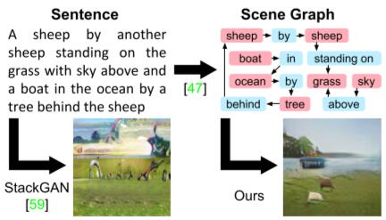
Previous work only performs well on limited domains such as followers or birds, but struggle to generate complex sentences with many objects and relationships.
This paper proposes a method for generating images from scene graphs with graph convolution which enable reasoning about objects and their relationships.
Method
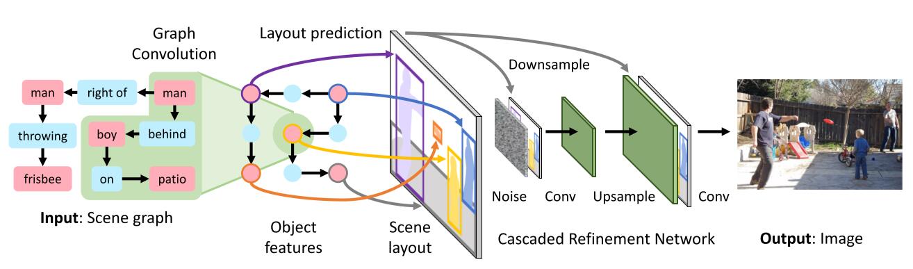
In summary, image generation network $f$ takes a scene graph $G$ and noise $z$ as input and outputs and image $\hat{I}=f(G, z)$.
Firstly, embedding vectors representing objects and edges were generated from graph convolution network, which is then concatenated to predict bounding boxes and segementation masks for each predicted object.
After obtaining the scene layout, which contains several bounding-boxes and masks, this high-dimensional representation is fed into cascaded refinement network TODO combined with noise to generate the final result.
Scene graph
As the first stage of processing, each node and edge of the graph from the dataset is converted to a dense vector by an embedding layer, analogous to the embedding layer which is used to get word-embeddings in neural language model.
Graph Convolution Network
A 2D convolution layer takes the above vectors as an input, and produces the output vectors with neighbourhood information of its corresponding input vector. In this way, convolution operation aggregates the information across the neighbourhood of the input.
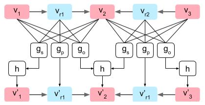
As the picture shown and concretely speaking, the output vectors $v_{i}^{\prime}$ for edges is simply computed by $v_{r}^{\prime}=g_{p}\left(v_{i}, v_{r}, v_{j}\right)$, while the calculation of objects vectors is a bit more complicated since the same object may participate in many relationships, e.g. A car is on the street. The street is besides the buildings. where ‘street’ acts as the starting node in the first edge while being the ending node in the second.
To this end, $g_{s}$ and $g_{o}$ is used to compute a candidate vector:
\[\begin{array}{l}{V_{i}^{s}=\left\{g_{s}\left(v_{i}, v_{r}, v_{j}\right) :\left(o_{i}, r, o_{j}\right) \in E\right\}} \\ {V_{i}^{o}=\left\{g_{o}\left(v_{j}, v_{r}, v_{i}\right) :\left(o_{j}, r, o_{i}\right) \in E\right\}}\end{array}\]Then the ouput vector $v_{i}^{\prime}$ for object is computed as $v_{i}^{\prime}=h\left(V_{i}^{s} \cup V_{i}^{o}\right)$ where $h$ is a symmetric function TODO.
Scene layout
After embedding vectors for objects was obtained, which aggregates all information across all objects and relationships in the edge, scene layout will be calculated to give the coarse 2D location information.
As below image shown, mask regression network and box regression network are built to predict a soft binary mask and a bounding-box respectively. The previous consists of several transpose convolutions terminating in sigmoid nonlinear function so that the mask lies in the range $(0,1)$ while the second is a MLP.
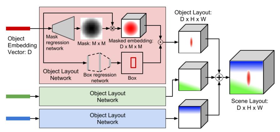
The mask embedding of shape $D \times M \times M$ TODO
Cascaded refinement network
This network consists of a series of convolutional refinement modules, doubling the resolution and proceeding in a corase-to-fine manner.
Each module receives both the scene layout and the output from the prvious module as its input, concatenated them channelwise, upsampling them with nearest-neighbor interpolation and then passing it to the next, and finally generate the output result.
Training
Discriminator
A pair of discriminator is built.
-
The patch-based image discriminator TODO $D_{img}$ ensures the overall appearance of generated images are realistic.
-
The object discriminator $D_{obj}$ has two functions:
-
ensuring objects in the image appears realistic by taking picels of object as inputs.
-
ensuring each object is recognizable by an auxiliary classifier to predict category.
-
Loss
The loss consists of six components.
-
Box loss $\mathcal{L}_{b o x}=\sum_{i=1}^{n}\left\|b_{i}-\hat{b}_{i}\right\|_{1}$ penalizing the $L_{1}$ distance between ground-truth and predicted boxes.
-
Mask loss $\mathcal{L}_{\text { mask }}$ penalizing differences between ground-truth and predicted masks with pixelwise cross-entropy.
-
Overal pixel loss $\mathcal{L}_{p i x}=\|I-\hat{I}\|_{1}$ penalizing the $L_{1}$ distance between ground-truth and generated images.
-
Image adversarial loss $\mathcal{L}_{G A N}^{i m g}$ from $D_{img}$ encouraging generated image patches to appear realistic.
-
Object adversarial loss $\mathcal{L}_{G A N}^{o b j}$ from $D_{obj}$ encouraging each generated object to look realistic.
-
Auxiliarly classifier loss $\mathcal{L}_{A C}^{o b j}$ from $D_{obj}$ ensuring each generated object can be classified by $D_{obj}$.
Conclusion
Compared to previous work, this paper uses structured text description to reason more explictly about objects and its relationships and generate more complex images with multiple objects.