Deep Generative Model, Basic thoery of GAN, Comparison to VAE, Equation derivations
Basic Idea of GAN
-
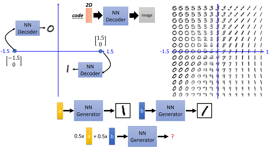
Each dimension of input vector represents some characteristic, which means that change the input of the noise, some of the characteristic of the output image will change.
-
The outout of discriminator is commonly a scalar. The larger value means realistic, while smaller means fake.
Algorithm
Algorithm Initialize $\theta_{d}$ for $\mathrm{D}$, and $\theta_{g}$ for $\mathrm{G}$
- In each training iteration:
- Sample m examples $\{ x^{1}, x^{2}, \ldots, x^{m} \}$ from database
- Sample m noise samples $\{z^{1}, z^{2}, \ldots, z^{m}\}$ from a distribution
- Obtaining generated data $\{\tilde{x}^{1}, \tilde{x}^{2}, \ldots, \tilde{x}^{m}\}, \tilde{x}^{i}=G\left(z^{i}\right)$
- Update discriminator paramters $\theta_{d}$ to maximize
\(\begin{aligned} &\tilde{V}=\frac{1}{m} \sum_{i=1}^{m} \log D\left(x^{i}\right)+\frac{1}{m} \sum_{i=1}^{m} \log \left(1-D\left(\tilde{x}^{i}\right)\right) \\ &\theta_{d} \leftarrow \theta_{d}+\eta \nabla \tilde{V}\left(\theta_{d}\right) \end{aligned}\) - Sample m noise samples $\{z^{1}, z^{2}, \ldots, z^{m}\}$ from a distribution
- Update generator parameters $\theta_{g}$ to maximize
\(\begin{aligned} &\tilde{V}=\frac{1}{m} \sum_{i=1}^{m} \log \left(D\left(G\left(z^{i}\right)\right)\right) \\ &\theta_{g} \leftarrow \theta_{g}-\eta \nabla \tilde{V}\left(\theta_{g}\right) \end{aligned}\)
- Takeaway:
- Fix generator G, update discriminator D. Discriminator learns to assign high scores to real objects and low scores to generated result. Gradient descent of the final score.
- Fix discriminator D, and update generator G. Gnerator learns to fool the discriminator. Gradient ascent of the final score.
Generator
- Generator can be designed as autoencoder
- Encoder part of the generator maps the original images to the latent space as the compact representation of the input object.
- Decoder part of the generator reconstructs the original object from code to generated result as closely as possible.
- After the training, we can discard the encoder part, replacing it with the input code as whatever we want.
- Change the input vector of the input noise, the generated result will vary smoothly, but may not make sense e.g. linear interpolation of the input noise
TODO VAE
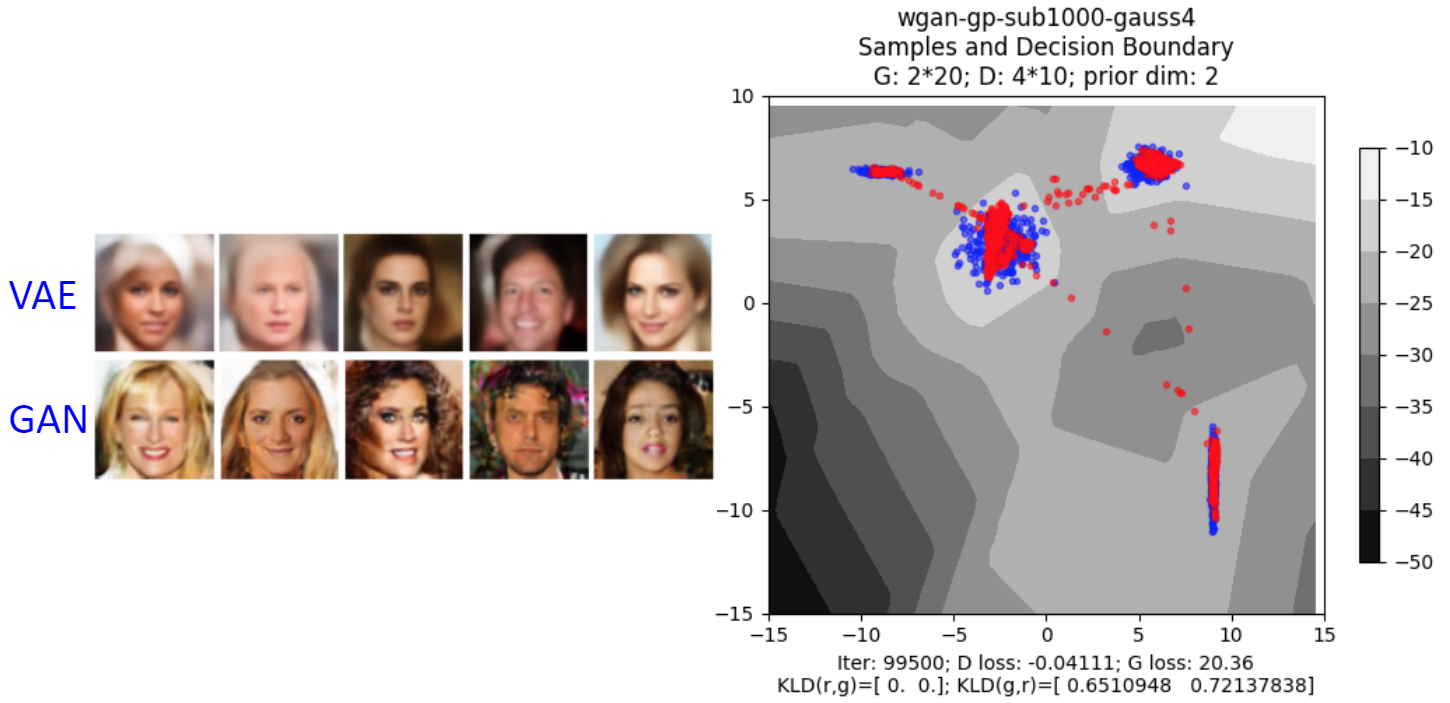
Comparing to VAE
TODO TODO result in what?
- VAE: The relation between components are not-correlated since neurons in the same layer of the network will not influence each other and they are independent
- Thus VAE can not discriminate naunced between features, which cause the result more vague than GAN
- To catch the correpondence among pixels, deep structure needed.
Discriminator
- Use discriminator to generate?
- Inference: Generate object $\widetilde{x}$ that
\(\widetilde{x}=\arg \max _{x \in X} D(x)\) - Enumerate all possible $x$, which is not always feasible, because the above equations can only be solved when it is linear. However linearity constrain the ability of the network.
- Inference: Generate object $\widetilde{x}$ that
- Algorithm:
- Given a set of positive examples and negative example generated randomly
- In each iteration
- Learn a discriminator D that can discriminate positive and negative examples
- Find relatively good examples from negative examples by $\widetilde{x}=\arg \max _{x \in X} D(x)$
- Replace the negative examples with relatively good examples
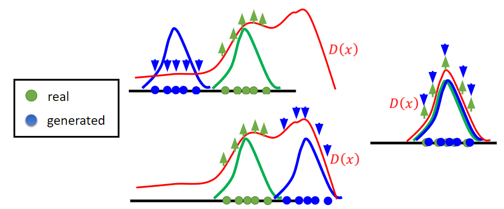
- From the above figure, we noticed that discriminator can only optimize the distribution corresponding to the generated distribution, which is one of the reason why GAN is difficult to optimize.
TODO structured learning
GAN
- From Discriminator’s point of view
- Use Generator to generate negative samples, replacing infeasible sovled
argmaxfunction
- Use Generator to generate negative samples, replacing infeasible sovled
- From Generator’s point of view
- Still generate the object without correspondence (pixel-by-pixel)
- But it is led by the instruction of the discriminator with global view
Basic Theory
Generation
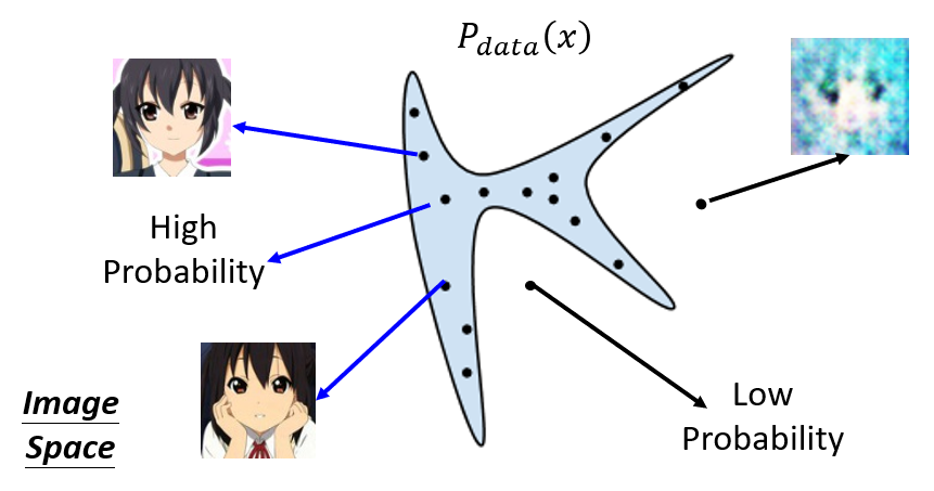
- The realistic images from dataset can be regarded as the low-dimensional manifold in high-dimensional space. Sampling from the dataset is the process of sampling from the manifold in the space.
Info: Manifold, in short, generalizes the triangle, circle, squares, etc. to higher dimensions. If we take a closer look at the N-dimensional manifold (N-manifold), it looks like N-1 dimensional manifold.
-
The ensemble of images from the sampling constitute the data distribution $P_{data}(x)$, which only occupies the tiny part of the whole high-dimensional space.
-
The point outside of the manifold means there will be low probablity of the true sampling.
-
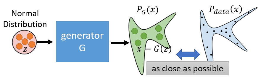
Building a generator is the process of building a mapping from one known distribution to the data distribution in high level.
Maximum Likelihood Estimation
- Target
- Given a data distribution $P_{data}(x)$
- We target at a distribution $P_{G}(x;\theta)$ parameterized by $\theta$
- To find $\theta$ such that $P_{G}(x;\theta)$ closed to $P_{data}(x)$
- e.g. if we assume $P_{G}(x;\theta)$ is Guassian Mixture Model, $\theta$ are means and variances of the Gaussians
- Step
- Derive $\{ x^{1}, x^{2}, \ldots, x^{m} \}$ by sampling from $P_{data}(x)$
- We can compute corresponding $P_{G}(x^{i};\theta)$
- Then find $\theta^{\ast}$ maximizing the likelihood
- Maximum Likelihood Estimation = Minimize KL Divergence
- KL-divergence measures the difference between two distribution $P_{\text {data}}$ and $P_{\text {G}}$
\(\begin{aligned} KL\left(P_{\text {data}} \| P_{G}\right) &= P_{\text {data}} \log P_{data}- P_{data} \log P_{\text {G}} \\[8px] &= P_{\text {data}} \log \frac{P_{data}}{P_{\text {G}}} \end{aligned}\) - $x \sim data$ means $x$ is sampled from the distribution of data.
- $P_{data}(x)$ means the probablity of the distribution
dataat $x$ sampling point. - $P_{G}(x;\theta)$ means the probablity of the distribution
Gat $x$ sampling point with parameter $\theta$.
- KL-divergence measures the difference between two distribution $P_{\text {data}}$ and $P_{\text {G}}$
TODO: Expectation Maximum
- What if $P_G$ is not Gaussian Mixture Model but more complex and general model?
- The mean and variance of the more complex model is difficult to get, since the explicit expression of the corresponding probability density function is unknown.
- Thus parameters $\theta$ are implicit and impossible to found.
Drawback of GMM
- In the past, Generator is built as Guassian Mixture model (GMM) with explicit parameters $\theta$.
- As mentioned before, GMM fails to represent the low-dimensional manifold which images lie along in high-dimensional space.
- Therefore, no matter what
meanandvarianceof GMM looks like, it fails to resemble the target distribution. - As a result, the output of GMM is obscure and fuzzy.
Generator
- Generator
Gis a network, which defines a probability distirbution $P_G$, mapping the input distribution to the target.- The network has an ability to approximate any functions.
- The input distribution is not decisive, normal distribution, uniform distribution, etc.
- Even the simplest distribution of input $z$ can be mapped to the complex one.
- The explicit formulations of $P_G$ and $P_{data}$ are still unknown, so it is impossible to do gradient descent on $G$ to minimize divergence.
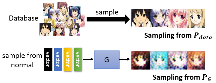
- But we can sample data from two distribution $P_G$ and $P_{data}$.
- Sampling from $P_{data}$: randomly sample from the database.
- Sampling from $P_G$: randomly sample from normal, fed into the network and get outputs.
- How to compute the divergence between samplings from two distributions? Discriminator
- But we can sample data from two distribution $P_G$ and $P_{data}$.
Info: Div is the divergence between two distribution, e.g. KL-divergence, JS-divergence.
Discriminator
-
Recall the objective function for generator
G:
\(G^{*}=\arg \min _G \operatorname{Div}\left(P_{G}, P_{\text {data}}\right)\) - The objective function for discriminator
D:
\(D^{*}=\arg \max _D \operatorname{V}(D, G) \\ V(G, D)=E_{x \sim P_{\text {data}}}[\log D(x)]+E_{x \sim P_{G}}[\log (1-D(x))]\) - This is exactly same as training a Binary Classifier
- $P_{data}$ is binary class
1 - $P_G$ is binary class
0 Dis a binary classifier- Binary classifier is to maximize Cross Entropy rather than Mean Square Error, since MSE-based objective is non-convex optimization problem
- $P_{data}$ is binary class
- The maximum objective is related to JS divergence.
- Given
G, the optimal $D^*$ maximizing:
\(\begin{aligned} D^{*}&=\arg \max _D \operatorname{V}(D, G) \\[10px] V(G, D) &=E_{x \sim P_{\text {data}}}[\log D(x)]+E_{x \sim P_{G}}[\log (1-D(x))] \\[10px] &=\int_{x} P_{d a t a}(x) \log D(x) d x+\int_{x} P_{G}(x) \log (1-D(x)) d x \\[10px] &=\int_{x}\left[P_{d a t a}(x) \log D(x)+P_{G}(x) \log (1-D(x))\right] d x \end{aligned}\) - Assume that
D(x)can represent any function.- Consider the integral as the sum of each piecewise function(分段函数) for $x_1, x_2, …$, since we have assumed
D(x)can represent any function, and neural network indeed can be regarded as piecewise function mathematically. - When each piecewise function reaches the largest individually, the final integral must also be the largest.
- Consider the integral as the sum of each piecewise function(分段函数) for $x_1, x_2, …$, since we have assumed
- Discretize the above equation, then the objective will be:
\(\begin{cases} P_{d a t a}(x) \log D(x)+P_{G}(x) \log (1-D(x)) \\[10px] a = P_{data},\ b = P_{G} \end{cases}\)- Solve for the extremum point:
\(\begin{aligned} \mathrm{f}(D) &=\operatorname{alog}(D)+b \log (1-D) \\[8px] \frac{d \mathrm{f}(D)}{d D} &=a \times \frac{1}{D}+b \times \frac{1}{1-D} \times (-1) =0 \\[8px] a \times\left(1-D^{*}\right) &=b \times D^{*} \\[5px] 0< D^{*} &=\frac{a}{a+b} =\frac{P_{\text {data}}(x)}{P_{\text {data}}(x)+P_{G}(x)}<1 \\[8px] 0< D^{*} &<1 \end{aligned}\)
- Solve for the extremum point:
- Substitue the optimal $D^* = \frac{P_{\text {data}}(x)}{P_{\text {data}}(x)+P_{G}(x)}$:
\(\begin{aligned} V &=E_{x \sim P_{\text {data}}}[\log D(x)]+E_{x \sim P_{G}}[\log (1-D(x))] \\[15px] &=E_{x \sim P_{\text {data}}}\left[\log \frac{P_{\text {data}}(x)}{P_{\text {data}}(x)+P_{G}(x)}\right]+E_{x \sim P_{G}}\left[\log \frac{P_{G}(x)}{P_{\text {data}}(x)+P_{G}(x)}\right] \\[15px] &=\int_{x} P_{\text {data}}(x) \log \frac{P_{\text {data}}(x)}{P_{\text {data}}(x)+P_{G}(x)} d x+\int_{x} P_{G}(x) \log \frac{P_{G}(x)}{P_{\text {data}}(x)+P_{G}(x)} d x \\[15px] &=\int_{x} P_{\text {data}}(x) \log \frac{\frac{1}{2}P_{\text {data}}(x)}{\frac{1}{2}[P_{\text {data}}(x)+P_{G}(x)]} d x+\int_{x} P_{G}(x) \log \frac{\frac{1}{2}P_{G}(x)}{\frac{1}{2}[P_{\text {data}}(x)+P_{G}(x)]} d x \\[15px] &=-2log2 + \int_{x} P_{\text {data}}(x) \log \frac{P_{\text {data}}(x)}{\frac{1}{2}[P_{\text {data}}(x)+P_{G}(x)]} d x+\int_{x} P_{G}(x) \log \frac{P_{G}(x)}{\frac{1}{2}[P_{\text {data}}(x)+P_{G}(x)]} d x \\[15px] &=-2log2 + K L\left(P_{\text {data}} \| \frac{P_{\text {data}}(x)+P_{G}(x)}{2}\right) + K L\left(P_{\text {G}} \| \frac{P_{\text {data}}(x)+P_{G}(x)}{2}\right) \\[15px] &=-2log2 + \color{red}{2JS\left(P_{\text {data}} \| P_{\text {G}}\right)} \end{aligned}\)
- JS divergence is symmetric, while KL divergence is asymmetric. \(\begin{aligned} JS\left(P_{\text {data}} \| P_{G}\right) &= \frac{1}{2}[KL(P_{\text {data}} \| M) + KL(P_{\text {G}} \| M)] \\ M &= \frac{1}{2}(P_{data} + P_{G}) \end{aligned}\)
TODO: inverse KL divergence
GAN
- The objective of Generator
Gis to minimize the divergence between $P_G$ and $P_{data}$ - The divergence is measured by Discriminator
D, which maximizes the cross entropy as a binary classifier. - The maximum objective is related to JS divergence.
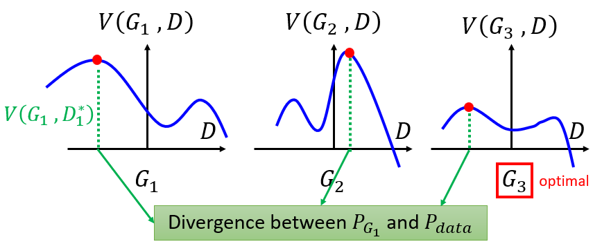
- For each fixed generator, we can find a discriminator with the maximum $V(D, G_i)$
- For each $V(D, G_i)$, we can get a minimum generator
- In each iteration
- Fix generator
G, update discriminator $D$. - Fix discriminator
D, update generator $G$.
- Fix generator
Algorithm
- To find the best
Gminimizing the loss function
\(G^{*}=\arg \min _G \max _D \operatorname{V}(D, G) = \arg\min_G L(G)\\ \theta_{G} \leftarrow \theta_{G}-\eta \partial L(G) / \partial \theta_{G}\)- Let the maximum value $\max_D V(G,D)$ as $L(G)$
- $\theta_G$ defines
G - The gradient of the max function is the gradient of max value of each piecewise function.
- Given $G_0$
- Find $D^*_0$ maximizing $V(G_0, D)$ , using Gradient Ascent
- $V(G_0, D_{0}^{*} )$ is the JS divergence between $P_data(x)$ and $P_{G_0}(x)$
- Obtain $G_1$
\(\theta_{G} \leftarrow \theta_{G}-\eta \partial V\left(G, D_{0}^{*}\right) / \partial \theta_{G}\) - Give $G_1$
- Find $D^*_0$ maximizing $V(G_0, D)$ , using Gradient Ascent
- $V(G_1, D_1^*)$ is the JS divergence between $P_data(x)$ and $P_{G_0}(x)$
- Obtain $G_2$ \(\theta_{G} \leftarrow \theta_{G}-\eta \partial V\left(G, D_{1}^{*}\right) / \partial \theta_{G}\)
Critical: Actually, after we get the optimal $D_i^*$ by maximizing the JS-divergence, given the fixed $G_i$, we do gradient descent optimizing $G_i$ a little bit per step to finally get $G_{i+1}$. However, in the process of the gradient descent of $G_i$ to $G_{i+1}$, the divergence function $V(G_i, D_i)$ may change a lot, which cause the maximum objective value of JS-divergence shift to somewhere else.
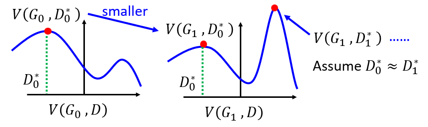
- Therefore, the important thing is that we don’t update $G$ too much for every steps, and $D$ is well-trained comparing to current $G$, so that the function of $V(G_i, D_i)$ won’t change a lot and $D_i^* \approx D_{i+1}^*$.
In practical
- Actually, We can not get the expectation value of $P_{data}$ or $P_G$
- In other words, we can not calculate the maximum value of the below equation:
\(V =E_{x \sim P_{\text {data }}}[\log D(x)]+E_{x \sim P_{G}}[\log (1-D(x))]\)
- In other words, we can not calculate the maximum value of the below equation:
- But we can do sampling from $P_{data}$ or $P_G$ to approximate the expectation.
- Given $G$, to compute $\max_D V(G,D)$
- Sample ${\tilde{x}^{1}, \tilde{x}^{2}, \ldots, \tilde{x}^{m}}$ from $P_{data}(x)$, sample ${x^{1}, x^{2}, \ldots, x^{m}}$ from generator $P_G(x)$
- To maximize:
\(\tilde{V}=\frac{1}{m} \sum_{i=1}^{m} \log D(x^{i})+\frac{1}{m} \sum_{i=1}^{m} \log (1-D(\tilde{x}^{i}))\)
- Thus, $D$ is a binary classifier with sigmoid output, which can be designed to be very deep.
- ${\tilde{x}^{1}, \tilde{x}^{2}, \ldots, \tilde{x}^{m}}$ from $P_{data}(x)$ is
Positive examples. - ${x^{1}, x^{2}, \ldots, x^{m}}$ from generator $P_G(x)$ is
Negative examples. - This is equivalent to minimize Cross-entropy.
- ${\tilde{x}^{1}, \tilde{x}^{2}, \ldots, \tilde{x}^{m}}$ from $P_{data}(x)$ is
Total Algorithm
Conclusion
- In each training iteration:
- Learning D: find lower bound of $\max_D V(G,D)$ and repeat
ktimes for fully trained.- Sample
mexamples $\{ x^{1}, x^{2}, \ldots, x^{m} \}$ from database distribution $P_{data}(x)$. - Sample
mnoise samples $\{z^{1}, z^{2}, \ldots, z^{m}\}$ from the prior $P_{prior}(z)$. - Obtaining generated data $\{\tilde{x}^{1}, \tilde{x}^{2}, \ldots, \tilde{x}^{m}\}, \tilde{x}^{i}=G\left(z^{i}\right), \tilde{x}^i = G(z^i)$.
- Update discriminator paramters $\theta_{d}$ to maximize.
\(\begin{aligned} &\tilde{V}=\frac{1}{m} \sum_{i=1}^{m} \log D\left(x^{i}\right)+\frac{1}{m} \sum_{i=1}^{m} \log \left(1-D\left(\tilde{x}^{i}\right)\right) \\ &\theta_{d} \leftarrow \theta_{d}\color{red}{+}\eta \nabla \tilde{V}\left(\theta_{d}\right) \end{aligned}\)
- Sample
- Learning G: find the minimum of $\min_G V(G,D)$ only once.
- Sample another
mnoise samples $\{z^{1}, z^{2}, \ldots, z^{m}\}$ from the prior $P_{prior}(z)$. - Update generator parameters $\theta_{g}$ to maximize
\(\begin{aligned} &\tilde{V}=\underset{\text{irrelevant to } G}{\boxed{\frac{1}{m} \sum_{i=1}^{m} \log D\left(x^{i}\right) } } +\frac{1}{m} \sum_{i=1}^{m} \log \left(D\left(G\left(z^{i}\right)\right) \right) \\ &\theta_{g} \leftarrow \theta_{g}\color{red}{-}\eta \nabla \tilde{V}\left(\theta_{g}\right) \end{aligned}\)
- Learning D: find lower bound of $\max_D V(G,D)$ and repeat
Note that it is impossible for $D$ to find the maximum value of $\max_D V(G,D)$, which means that the JS-divergence can never be reached, because:
1. The learning ability of $D$ is limited due to the iteration times and learning rate, the $D$ can not convergence in several update steps.
2. Even with the infinite training step and the convergence achieved, it is more likely for $D$ to fall in local minima.
3. Even without trapped in local minima, the capcity of the generatlization of $D$ is limited, which contradict the assumption that $D$ can represent all functions.
In Real Implementation
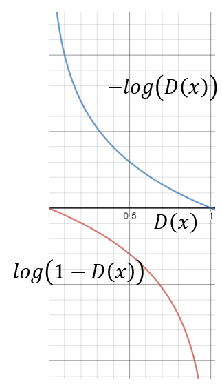
- The training of $G$ would be slow because of the initial output of $D(x)$ is closed to $0$ and the corresponding gradient to $G$ is very small. \(V =\underset{\text{irrelevant to } G}{\boxed{E_{x \sim P_{\text {data } }}[\log D(x)]}}+E_{x \sim P_{G}}[\log (1-D(x))]\)
- Two workarounds
- Replace the target with the following, greatly increase the gradient of the very beginning stage, Minimax GAN (MMGAN) \(V = E_{x \sim P_{G}}[- \log (D(x))]\)
- Replace the negative label of $G$ with the positive label, Non-saturating GAN (NSGAN)