Feature Extraction and Disentanglement

Feature Disentangle

The GAN receives one vector as input and output a desirable result.
- We hope to control the characteristic of the output by mopdifying each specific value in the input vector.
For general GAN, modifying a specific dimension of the vector commonly change the feature of the result unconsciously
- Because the actual distribution of each feature are intricate and entangled in the latent space.

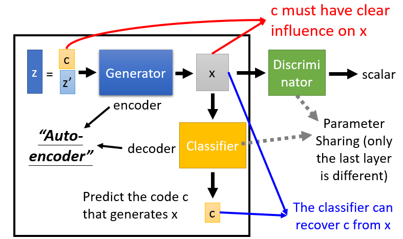
InfoGAN

Split input z to two parts, c encodes the different feature in each dimension and z' as input noise.
Classifier recover the predict c from the output x from the Generator, which supervises the generate to output x with the feature of c.
Discriminator still output a scalar to represent the result good or not, but shares the parameter with Classifier except for the last output layer.
- Without Discriminator, the output from Generator will only focus on c which benefit for the Classifier to predict, but generate bad results.

gan-4-1

*reference-2

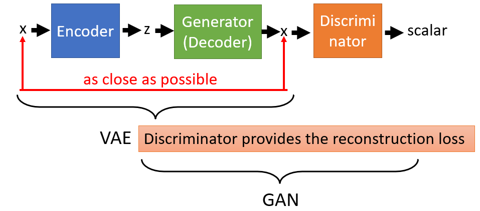
VAE-GAN

Based on VAE (variational auto-encoder), VAE-GAN combines VAE and GAN
- VAE only generates obscure results.
- Discriminator
Encoder is to encode the input image from the dataset to a normal distribution code z, regularized by imposing a prior distribution over the latent distribution $p(z)
Generator is to generate images and cheat the distriminator
- Output the reconstruction image from the output z of Encoder: minimize the reconstruction
- Output the generated image from the noise sampled from the prior distribution: get z as closed to the normal distribution as possible.
Discriminator is to distinguish the real, generated or reconstructed images.

Algorithm of the training the VAE-GAN

Initialize Enc, Dec, D

In each training iteration:

Sample m images $\{ x^{1}, x^{2}, \ldots, x^{m} \}$ from database distribution $P_{data}(x)$.
Generate m codes $\{\tilde{z}^{1}, \tilde{z}^{2}, \ldots, \tilde{z}^{m}\}$ from encoder, $\tilde{z}^i = Enc(x^i)$.
Generate m images $\{\tilde{x}^{1}, \tilde{x}^{2}, \ldots, \tilde{x}^{m}\}$ from decoder, $\tilde{x}^i = Dec(\tilde{z}^i)$.
Sample m noise samples $\{z^{1}, z^{2}, \ldots, z^{m}\}$ from the prior $P_{prior}(z)$.
Generate m images $\{\hat{x}^{1}, \hat{x}^{2}, \ldots, \hat{x}^{m}\}$ from decoder, $\hat{x}^i = Dec(z^i)$.

Update Enc to decrease reconstruction error of MSE $\lVert \tilde{x}^i - x^i \rVert$, decrease $\textit{KL-divergence}(P(\tilde{z}^i x^i) \Vert P(z))$

Update Dec to decrease reconstruction error of MSE $\lVert \tilde{x}^i - x^i \rVert$, increase binary cross entropy $D(\tilde{x}^i)$ and $D(\hat{x}^i)$.
Update D to increase binary cross entropy $D(x^i)$, decrease $D(\tilde{x}^i)$ and $D(\hat{x}^i)$.

gan-4-2

Info: Another kind of discriminator can be implemented to output three labels of the result: real, generated and reconstructed.

Algorithm of the training VAE-GAN

Initialize Enc, Dec, D

In each training iteration:

Sample m images $\{ x^{1}, x^{2}, \ldots, x^{m} \}$ from database distribution $P_{data}(x)$.
Generate m codes $\{\tilde{z}^{1}, \tilde{z}^{2}, \ldots, \tilde{z}^{m}\}$ from encoder, $\tilde{z}^i = Enc(x^i)$.
Generate m images $\{\tilde{x}^{1}, \tilde{x}^{2}, \ldots, \tilde{x}^{m}\}$ from decoder, $\tilde{x}^i = Dec(\tilde{z}^i)$.
Sample m noise samples $\{z^{1}, z^{2}, \ldots, z^{m}\}$ from the prior $P_{prior}(z)$.
Generate m images $\{\hat{x}^{1}, \hat{x}^{2}, \ldots, \hat{x}^{m}\}$ from decoder, $\hat{x}^i = Dec(z^i)$.

Update Enc to decrease reconstruction error of MSE $\lVert \tilde{x}^i - x^i \rVert$, decrease $\textit{KL-divergence}(P(\tilde{z}^i x^i) \Vert P(z))$

Update Dec to decrease reconstruction error of MSE $\lVert \tilde{x}^i - x^i \rVert$, increase binary cross entropy $D(\tilde{x}^i)$ and $D(\hat{x}^i)$.
Update D to increase binary cross entropy $D(x^i)$, decrease $D(\tilde{x}^i)$ and $D(\hat{x}^i)$.

Info: Another kind of discriminator can be implemented to output three labels of the result: real, generated and reconstructed.

*reference-3

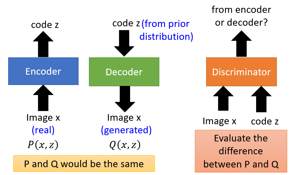
BiGAN

Make pair of the input and output from Encoder and Decoder to feed into the discriminator, distinguishing the the input come from the encoder or the decoder
Encoder takes the image x from the dataset and generate code z, and make a pair (x, z) (the corresponding distribution P(x, z)) for discriminator.
- Deceive Discriminator that the P(x, z) is from eecoder.
Decoder takes the code z' sampled from the prior distribution and generate image x', and make a pair (x', z) (the corresponding distribution Q(x', z')) for discriminator.
- Deceive Discriminator that the Q(x', z') is from dncoder.
Discriminator evaluate the difference between the distribution from encoder and decoder.
After the well training, the discriminator can not distinguish the distribution from encoder and decoder.
- P(x, z) will be the same as Q(x', z').
- The embedding code z will be similar to the code generated from the prior distribution, and the image x' from decoder will be real.
- The cycle consistency holds, which is similar to cycleGAN:
  - Also, Enc(x) = z => Dec(z') = x for all x'.
  - Similarly, Dec(z) = x => Enc(x) = z for all z.

gan-4-3

Algorithm of the training Bi-GAN
Initialize Enc, Dec, D
In each training iteration:
- Sample m images $\{ x^{1}, x^{2}, \ldots, x^{m} \}$ from database distribution $P_{data}(x)$.
- Generate m codes $\{\tilde{z}^{1}, \tilde{z}^{2}, \ldots, \tilde{z}^{m}\}$ from encoder, $\tilde{z}^i = Enc(x^i)$.
- Sample m noise samples $\{z^{1}, z^{2}, \ldots, z^{m}\}$ from the prior $P_{prior}(z)$.
- Generate m images $\{\tilde{x}^{1}, \tilde{x}^{2}, \ldots, \tilde{x}^{m}\}$ from decoder, $\tilde{x}^i = Dec(z^i)$.
- Update D to increase $D(x^i, \tilde{z}^i)$, decrease $D(\tilde{x}^i, z^i)$.
- Update Enc to decrease $D(x^i, \tilde{z}^i)$.
- Update Dec to increase $D(\tilde{x}^i, z^i)$.

Note: It doesn’t matter that the D gives the positive score to the pair from Enc or another. What matters is that the score D gives to Enc or Dec should be opposite. The objective of Enc and Dec should also be the opposite of the objective of D so that D could not discriminate between the generated pair after the advesarial training.

Based on the self-supervised way ofBiGAN, cycleGAN introduces the cycle consistency loss.

*reference-4

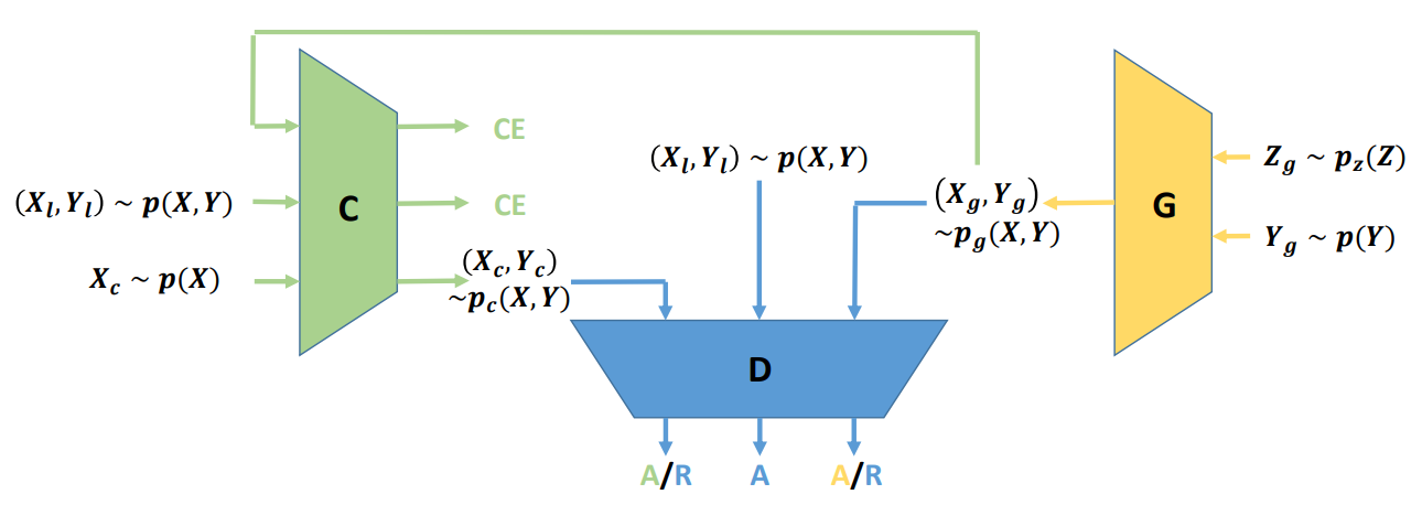
Triple GAN

Semi-supervised learning way of training GAN consists of three parts: classifier, generator, discriminator.
Generator receives the sampling noise $Z_g$ and conditional distribution $Y_g$ from the prior distribution, and output the pair of the image with the label $(X_g, Y_g)$
Classifier outputs the label of the image,and disentangle the class and style of the input in both supervised and unsupervised way:
- Take the output image-label pairs from generator, calculate the cross entropy reconstruction loss between predicted label $\tilde{Y}_g$ with $Y_g$. This process is using weak self-supervised sample to train the classifier.
- Take sampling pair $(X_l, Y_L)$ from the dataset and supervised learning with the cross entropy reconstruction loss between the predicted $\tilde{Y}_l$ and $Y$.
- Classify sampling image $X_c$ as the predicted label $Y_c$. The predicted pair is sent to the discriminator.
Discriminator solely identifies fake image-label pairs.
- Distinguish the real image-label pair sampled from the dataset directly.
- Distinguish the generated image-label pair from the generator.
- Distinguish the image and predicted label pair from the classifier.

gan-4-4

*reference-5

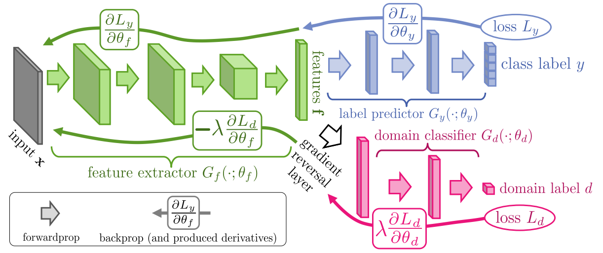
Domain-adversarial Training

The network consists of three parts:
- Feature extractor: extract and map the input $x$ to the latent space.
  - To maximize label classification accuracy
  - To minimize domain lcassification accuracy
- Label predictor: predict the class label of the feature from the extractor.
  - To maximize label classification accuracy
- Domain classifier: classify the source domain of the feature from the extractor.
  - To maximize domain classification accuracy
Gradient reversal layer is an identity function during the forward propagation, but it multiplies its input by -1 during backpropagation.
- Because it leads the gradient ascent on the feature extractor with respect to the classification loss of Domain predictor, but gradient descent on the predictor itself.

gan-4-5

*reference-6

Feature Disentangle

The encoding from the original encoder includes mixture information, which is entangled.
Embedding audio signal can be roughly classified as two parts
- Phonetic information: audio content, structures and semantic meaning
- Speaker information: audio speaker acoustic characteristics
Utilize two encoder to disentangle the above two information in the latent space: Phonetic encoder and Speaker encoder.

gan-4-6

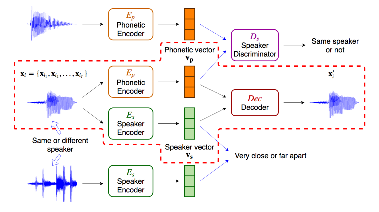
For the audio source from the same or different speakers, the speaker vector $v_s$ from Speaker Encoder $E_s$ will be constrained as close or far apart as possible.
- To guide the Speaker Encoder $E_s$ only extract the acoustic characteristic to the speaker vector $v_s$.
For inputs with different content and structures, the Phonetic Encoder $E_p$ embedding the Phonetic vector $v_p$, which is fed into Speaker Discriminator $D_s$ to distinguish if the source is from the same speaker or not.
- To instruct the Phonetic Encoder $E_p$ embeds all information except for the speaker characteristic.
Speaker Classifier $D_s$ is inspired from domain adversarial training, which outputs the score, representing how confident the discriminator $D_s$ will be that two audio source are from the identical speaker.
- The higher score means more confident on the same speaker.
- Phonetic encoder $E_p$ learns to confuse Speaker Classifier $D_s$.
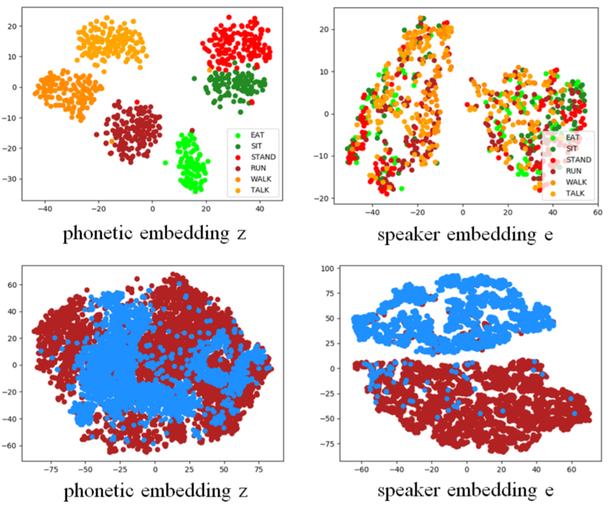
- After the well training, $D_s$ fail to distinguish whether the source is from the same speaker or not, and $E_p$ only generates embeddings with phonetic information.

gan-4-7

*reference-7

Each dimension of the input vector represents some characteristics, but the explicit relationship is unknown.
- Disentangle: understand the meaning of each dimension so as to control the output.

Attribute Modification

Compute the center of each sampling with the same attributes and compute the distance between different sampling centers.

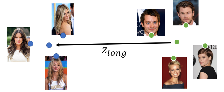
\[z_{\text {long }}=\frac{1}{N_{1}} \sum_{x \in \text { long }} \operatorname{En}(x)-\frac{1}{N_{2}} \sum_{x^{\prime} \notin \text { long }} \operatorname{En}\left(x^{\prime}\right)\]

gan-4-8

Transform the characteristic by compensating the distance in the latent space.

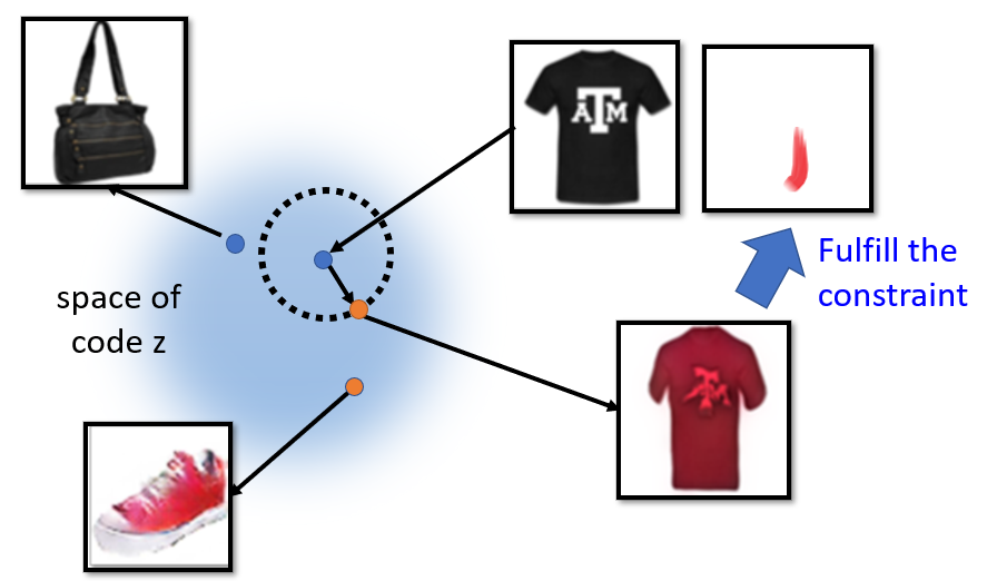
\[x \Rightarrow \operatorname{En}(x)+z_{\text {long }}=z^{\prime} \Rightarrow \operatorname{Gen}\left(z^{\prime}\right)\]

Photo Editing

Basic idea: find the optimum code $z^*$ in the latent space, closed to the original input image, at the same time fulltill the constraint.

gan-4-9

Three methods to backtrace code $z^*$ from the input $x$:
1. Gradient descent to find the optimal target:
  $z^{*}=\arg \min _{z} L\left(G(z), x\right)$
  The difference between $G(z)$ and $x$ can be measured by:
- Pixel-wise distance
- Another extractor network to evaluate the high level distance
  1. Well-trained auto-encoder structure to extract the latent code, transforming the input image back.
  2. Using the result from method 2 as the initialization of method 1 and fine-tune.
Editing photos with input constraint:
- $z_0$ is the code of the input image previously found.
- $U$ is the function to judge if the final generation fulfill the constaint of the editing.
- $\left|z-z_{0}\right|$ make sure the result is not too far away from the original image.
- $D$ discriminator is to check the image realistic or not. $z^{*}=\arg \min _{z} U(G(z))+\lambda_{1}\left\|z-z_{0}\right\|^{2}-\lambda_{2} D(G(z))$

*reference-8 *reference-9

Others

TODO

Many tasks as Image super resolution, Image completion, etc. are based on condition GAN.

Reference

PREVIOUSSequence and Evaluation