Advanced Thoery and Problems of GAN

Drawback of the general framework of GAN, Wasserstein Distance, WGAN-GP

General Framework of GAN

F-divergence

• $P$ and $Q$ are two distributions. $p(x)$ and $q(x)$ are the probability of sampling $x$.
• f-divergence $D_{f}(P | Q)$ evaluates the difference of $P$ and $Q$.
  • $f$ is convex function
  • when $P$ and $Q$ are the same distributions, $p(x) = q(x)$, $f(\frac{p(x)}{q(x)}) = f(1) = 0$

\[\begin{aligned} D_{f}(P \| Q) &=\int_{x} q(x) f\left(\frac{p(x)}{q(x)}\right) d x \\ & \geq f\left(\int_{x} q(x) \frac{p(x)}{q(x)} d x\right) \color{red}{\text{Jessen Inequality}} \\ & = f\left(\int_{x}p(x) d x\right) \\ & = f(1) \\ & = 0 \end{aligned}\]

Note: Considering $f$ is the convex function, the above inequation can be established according to Jessen inequation:
$ \varphi\left(\frac{1}{b-a} \int_{a}^{b} f(x) d x\right) \leq \frac{1}{b-a} \int_{a}^{b} \varphi(f(x)) d x $

• f function can be different

\[\begin{aligned} &\text{When } f(x)=x \log x \text{ , KL-divergence:}\\ &D_{f}(P \| Q)=\int_{x} q(x) \frac{p(x)}{q(x)} \log \left(\frac{p(x)}{q(x)}\right) d x=\int_{x} p(x) \log \left(\frac{p(x)}{q(x)}\right) d x \\[1em] &\text{When }f(x)=-\log x \text{ , reversed KL-divergence:}\\ &D_{f}(P \| Q)=\int_{x} q(x)\left(-\log \left(\frac{p(x)}{q(x)}\right)\right) d x=\int_{x} q(x) \log \left(\frac{q(x)}{p(x)}\right) d x \\[1em] &\text{When }f(x)=(x-1)^{2} \text{ , Chi Square-divergence:}\\ &D_{f}(P \| Q)=\int_{x} q(x)\left(\frac{p(x)}{q(x)}-1\right)^{2} d x=\int_{x} \frac{(p(x)-q(x))^{2}}{q(x)} d x \end{aligned}\]

Fenchel Conjugate

• Fenchel Conjugate (Convex conjugate 凸共轭): the paired appearance of two functions with a strong relationship.
  • Duality (对偶) relationship is built on the same linear hyperplane.
• The purpose of using conjugate functions:
  • The advantage is that even if a function is not convex, a convexed function can be obtained by the conjugate method.
  • Even better, through the conjugation again, we can get a good approximation function with the original function.
  • The convex hull function of the original function can be obtained by conjugating twice, where many excellent properties of the new convex hull will be obtained in the optimization solution with just a little loss.
• Every convex function $f$ has a conjugate function $f^*$

\[f^{*}(t) =\max _{x \in \operatorname{dom}(f)}\{x t-f(x)\}\]

• The variable of $f^* (t)$ is $t$, and get the maximum for every possible value of $x$.

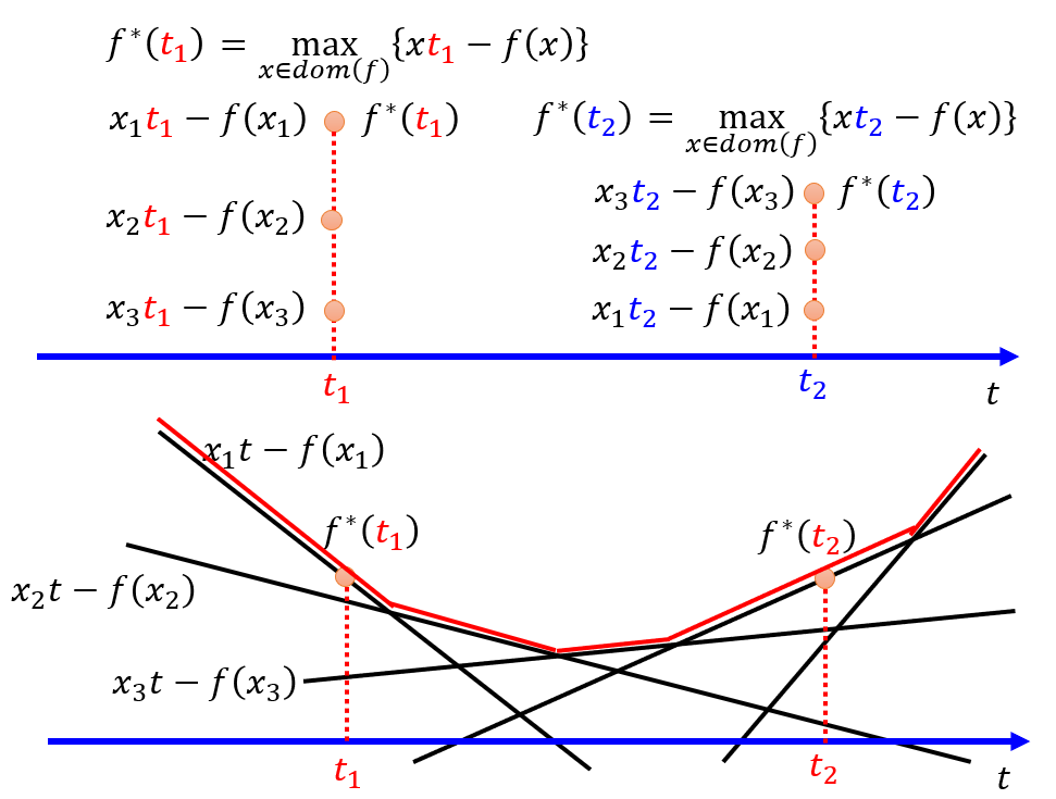
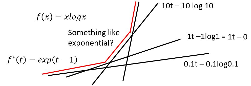
• We can get a good approximation function with the original function
  • E.g. $f(x) = xlogx$ can be approximated as $f^*(t) = e^{t-1}$.

\[\begin{aligned} &\text{Take } f(x) \text{ as } xlogx \text{ :}\\ &\quad f^{*}(t) =\max _{x \in \operatorname{dom}(f)}\{x t-f(x)\} = \max _{x \in \operatorname{dom}(f)}\{x t-x \log x\}\\ &\text{Let } g(x) =x t-x \log x \text {, Given } t, \text { find } x \text { to maximize } g(x) \text{:}\\ &\quad t-\log x-1=0 \quad \\ &\quad x= e^{t-1} \\ &\quad f^{*}(t)= e^{t-1} \times t-e^{t-1} \times(t-1)=e^{t-1} \\ \end{aligned}\]

Connection with GAN

• Derivation of GAN’s derivation:
  • From the convex conjugate:
    \(f^{*}(t)=\max _{x \in \operatorname{dom}(f)}\{x t-f(x)\} \longleftrightarrow f(x)=\max _{t \in \operatorname{dom}\left(f^{*}\right)}\left\{x t-f^{*}(t)\right\}\)

  • Take $x$ as $\frac{p(x)}{q(x)}$ :
    \(\begin{aligned} D_{f}(P \| Q) &=\int_{x} q(x) f\left(\frac{p(x)}{q(x)}\right) d x \\ &=\int_{x} q(x)\left(\max _{t \in \operatorname{dom}\left(f^{*}\right)}\left\{\frac{p (x)}{q(x)} t-f^{*}(t)\right\}\right) d x \\ &\color{red}{\geq} \int_{x} q(x)\left(\frac{p(x)}{q(x)} \color{red}{D(x)}-f^{*}( \color{red}{D(x)})\right) d x \\ &=\int_{x} p(x) D(x) d x-\int_{x} q(x) f^{*}(D(x)) d x \\ \end{aligned}\)

  • The reason of replacing $\max$ item with $D(x)$ as above in red color:
    • $D(x)$ takes $x$ as input and output $t$.
    • The limited capcity of $D$ determines the lower bound of $\max$ item.

  • For the divergence between $P$ and $Q$:
    \(\begin{aligned} D_{f}(P \| Q) &\approx \max _{\mathrm{D}} \int_{x} p(x) D(x) d x-\int_{x} q(x) f^{*} (D(x)) d x \\ &=\max _{\mathrm{D}}\left\{E_{x \sim P}[D(x)]-E_{x \sim Q}\left[f^{*}(D(x))\right] \right\} \\ &\quad\text { Samples from P } \quad \text { Samples from Q } \\ \end{aligned}\)

  • Convert the conjugate to the more general form of GAN’s objective by sampling from $P_{data}$ and $P_G$: \(D_{f}\left(P_{\text {data}} \| P_{G}\right)=\max _{\mathrm{D}}\left\{E_{x \sim P_{\text {data}}}[D(x)]-E_{x \sim P_{G}}\left[f^{*}(D(x))\right]\right\} \\ \begin{aligned} G^{*} &=\arg \min _{G} D_{f}\left(P_{d a t a} \| P_{G}\right) \\ &=\arg \min _{G} \max _{D}\left\{E_{x \sim P_{\text {data}}}[D(x)]-E_{x \sim P_{G}}\left[f^{*}(D(x))\right]\right\} \\ &=\arg \min _{G} \max _{D} V(G, D) \end{aligned}\)
    • Therefore, according to the different definition of $V(G,D)$, we can have different divergence, which corresponds to different $f^*$ function.

*reference-2

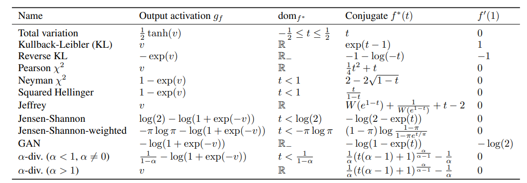
• What benefit we can get to try different divergence (and corresponding $f^*$ function)?

Mode Collapseand & Dropping

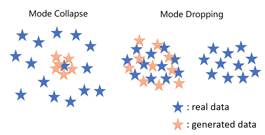
• Mode collapse and Mode Dropping refer to reduced variety in the samples produced by a generator.
  • Mode Collapse: The generator synthesizes samples with intra-mode variety, but some modes are missing.
    • E.g. Generator outputs limited variaty of faces with many duplicates.
  • Mode Dropping: The generator synthesizes samples with inter-mode variety, but each mode lacks variety.
    • E.g. Generator outputs various faces at once, but all with the same one feature, like white skins.

• The problem may be caused by the bad selection of divergence

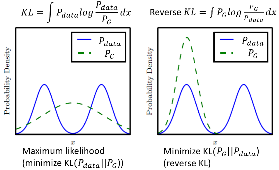
• As the below picture shows:

  • The left figure shows the problem of KL-divergence, where the distribution of the well-trained generator falls between the peak of the true data distribution.
    • This is also one explanation of why traditional generation, like autoencoder, output obscure result by choosing KL-divergence and minimizing it (aka. maximizing the likelihood estimation).
    • The distribution between the peak refers to those obscure generated images.
  • The right figure shows the mode collapse and dropping problem, where the trained distribution mainly lies in one single peak.
    • This is one explanation of why advesarial training often encounters the limited diversity or limited features problems.
    • The missing distribution of generator referes to the missing features.

• But choosing different divergence can not solve the problem completely.
  • One triky workarounds is train the different generator, each with limited diversity and mode collapse or dropping problems. Gather to be the better generator.

Improving GAN

Problem of JS-divergence

• In most cases $P_G$ and $P_{data}$ are not overlapped for the following reason:
  • The nature of data determines that $P_{data}$ and $P_G$ are low-dimensional manifold in high-dimensional space. Thus the overlap of two distribution can be ignored
  • Limited sampling cause that even though the distribution of $P_{data}$ and $P_G$ have overlap, the discriminator frequently fails to measure the divergence between the distribution of sampling which is still sparse without enough overlap.

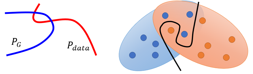
Info: Images are the low-dimensional manifold in high-dimensional space. If we hypothesis the space is only 3D, the images is a line or plane in this 3D space.

• Considering the objective of Discriminator: \(V(G,D)=-2log2 + \color{red}{2JS\left(P_{\text {data}} \| P_{\text {G}}\right)}\)
  • If there is nearly no overlap between two distribution, the value of JS-divergence would be 2log2 constant item, the gradient of which would be zero, which could cause the training stop.
  • And it is very common that two distribution have little overlap in high-dimensional space.
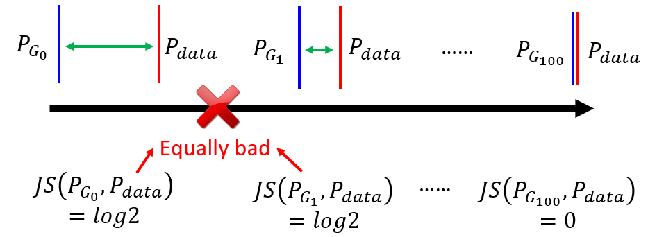
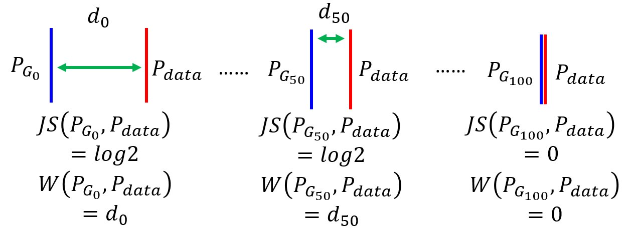
• As the following figure shows:
  • $P_{G_1}$ performs better than $P_{G_0}$ theoretically because it is closer to $P_{data}$, but the JS-divergence of two are all log2 (ignore the coefficient 2 ahead).
  • Only two distribution are exactly the same, the JS-divergence will be 0, which is the final target of generator.

Note: Strictly, according to the above equation of the objective of the discriminator, the JS-divergence is closed to 0 and the total objective is log2 if there is barely enough overlap between distributions.

• The generator is to minimize the divergence, but the same value log2 of the objective gives no guide for the generator to judge which situation is worse. In other words, $P_{G_0}$ and $P_{G_1}$ are considered equally bad. Therefore, the generator will not update from $P_{G_0}$ to $P_{G_1}$.
• On the other hand, the discriminator also consider $P_{G_0}$ and $P_{G_1}$ equally bad. Considering only when two distribution are exactly the same, JS-divergence is 0, binary classifier will always achieves 100% accuracy.

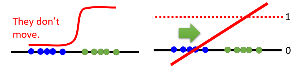
Most important: For the discriminator, a binary classifier, as long as the output of the classification is the false label, the loss is constant regardless of the deviation between the current $P_G$ and $P_{data}$. This property of JS-divergence makes it impossible to measure the distance between the non-overlapping distributions and hence the generator cannot be optimized properly.

LSGAN

• In the binary classifier point of view, the gradient vanishing occurs when generate distribution is distinguished as fake too well after the sigmoid nonlinear transform.
  • Low-dimensional manifold in the high-dimensional space has almost no overlap, so the discriminator can clearly classified into 0 and 1, so that the gradient vanishing concentrates at both ends.
• Least Square GAN (LSGAN): replace the sigmoid function with the linear, converting the binary classification problem into the regression problem.

Wasserstein GAN

Wasserstein Distance

• Instead of using divergence to measure the distance between distributions, Wasserstein GAN (WGAN) use Earth Mover’s Distance.
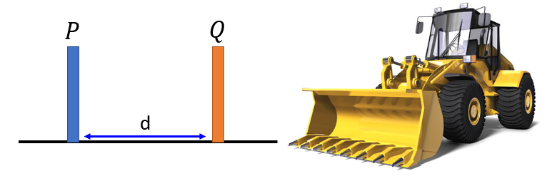
  • Consider one distribution $P$ as a pile of earth and another distribution $Q$ as the target.
  • Wasserstein Distance, also descriptively called Earth Mover’s Distance (EMD): the minimal total amount of work it takes to transform one heap into the other (initial distribution to the target).
    \(W(P, Q) = d\)
  • The work defines as the amount of earth in a chunk times the distance it was moved.

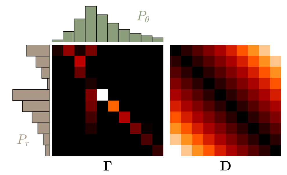
• Assume two discrete distributions $P_r$ and $P_{\theta}$, each with $l$ possible states $x$ or $y$ respectively.

• There are infinitely ways to move the earth around, but we only need to find the optimal one for EMD.

  • Denote $\gamma(x, y)$ as the amount of earth distributed from $x$ to the domain of $y$.
  • The constraints $\sum_{x} \gamma(x, y)=P_{r}(y)$ and $\sum_{y} \gamma(x, y)=P_{\theta}(x)$ holds.
  • We require that $\gamma \in \Pi (P_{r}, P_{\theta})$, where $\Pi (P_{r}, P_{\theta})$ is the set of all distributions whose margains are $P_r$, $P_{\theta}$ respectively.
  • We multiply every value of $\gamma$ with the Euclidian distance between $x$ and $y$.

\[\operatorname{EMD}\left(P_{r}, P_{\theta}\right)=\inf _{\gamma \in \Pi} \sum_{x, y}\|x-y\| \gamma(x, y)=\inf _{\gamma \in \Pi} \mathbb{E}_{(x, y) \sim \gamma}\|x-y\|=\inf _{\gamma \in \Pi}\langle\mathbf{D}, \mathbf{\Gamma}\rangle_{\mathrm{F}}\]

• $\inf$ stands for infimum, or the greatest lower bound (下确界), roughly meaning the minimum, the opposite of which is $\sup$ for supremum (上确界)
• The distribution strategy is set as $\mathbf{\Gamma}=\gamma(x, y)$, and distance is $\mathbf{D}=\lVert x-y \rVert$, with $ \boldsymbol{\Gamma}, \mathbf{D} \in \mathbb{R}^{l \times l} $, then the definition of EMD will be:
• ${\langle , \rangle}_{F}$ is the Frobenius inner product, the sum of all the element-wise products.

*reference-3

WGAN

• Instead of the Divergence $D_f (P_{data} \Vert P_G)$, which consider the generated distribution equally bad when there is not much overlap in space, the Wasserstein Distance $W(P_{data}, P_G)$ gives the exact distance function between $P_G$ and $P_{data}$

• By solving the optimization problem and finding the best $\gamma(x, y)$, we can evaluate wasserstein distance between $P_{data}$ and $P_G$:
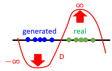
  • maximize the $D(x)$ where $x$ is from $P_{data}$
  • minimize the $D(x)$ where $x$ is from $P_G$

\[V(G,D) = \max_{D \in \textit{1-Lipschitz}} \left\{ E_{x \sim P_{\text {data}}} [D(x)] - E_{x \sim P_G} [D(x)] \right\}\]

TODO: the derivation.

• $D \in \textit{1-Lipschitz}$: D has to be smooth enough, so that the generated distribution and the real distribution will not be distinguished too much.
  • Without this constraint, the generated score will become small to $-\inf$, while the real will be large as $+\inf$, which will make network hard to train due to the large weight and never converge.
  • Thus, keep discriminator smooth is one way to keep the score from $\inf$.

• Lipschitz Continuity: the function limited how fast it can change.
  • When $ K = 1$ is $\textit{1-Lipschitz}$

\[\underset{\text{output change}}{\lVert f(x_1) - f(x_2) \rVert} \le K \underset{\text{input change}}{\lVert x_1 - x_2 \rVert}\]

• Weight Clipping: a simple but efficient way to enforce a Lipschitz constraint.
  • Force the parameters $w$ between $c$ and $-c$
  • After parameters update, $ \text{if } w \gt c, w = c, \text{if } w \lt -c, w = -c$

*reference-4

WGAN-GP

• WGAN-GP: Wasserstin GAN with the gradient penalty.
  • A differentiable function is 1-Lipschitz if and only if it has gradients with a norm less than or equal to 1 everywhere.

\[\begin{aligned} &D \in \textit{1-Lipschitz}\Longleftrightarrow \left\|\nabla_{x} D(x)\right\| \le 1, \quad \text{for all } x\\[8px] &\begin{aligned} V(G, D) &=\max _{D \in \textit { 1-Lipschitz }}\left\{E_{x \sim P_{\text {data}}}[D(x)]-E_{x \sim P_{G}}[D(x)]\right\} \\ & \approx \max _{D} \{E_{x \sim P_{\text {data}}}[D(x)]-E_{x \sim P_{G}}[D(x)] -\lambda \int_{x} \max _{x}\left(0,\left\|\nabla_{x} D(x)\right\|-1\right) d x\} \\ \end{aligned} \end{aligned}\]

• Instead of promising all constraints of the gradient for all $x$ because enforcing the Lipschitz constraint everywhere is intractable, we only guarantee $x \in P_{penalty}$.

\[\begin{aligned} V(G, D) & \approx \max _{D} \{E_{x \sim P_{\text {data}}}[D(x)]-E_{x \sim P_{G}}[D(x)] -\underset{\color{red}{\text{Prefer } \left\|\nabla_{x} D(x)\right\|\le 1, \text{ for all } x}}{\lambda \int_{x} \max _{x}\left(0,\left\|\nabla_{x} D(x)\right\|-1\right) d x}\} \\ & \approx \max _{D} \{E_{x \sim P_{\text {data}}}[D(x)]-E_{x \sim P_{G}}[D(x)] -\underset{\color{red}{\text{Prefer } \left\|\nabla_{x} D(x)\right\|\le 1, \text{ for } x \text{ sampling from } x \sim P_{penalty}}}{\lambda E_{x \sim P_{\text {penalty}}} [\max _{x}\left(0,\left\|\nabla_{x} D(x)\right\|-1\right)]} \} \end{aligned}\]

• By randomly sampling, enforcing the $x$ only along the straight lines, as following figure shows, is sufficient and experimentally results in good performance.
• Only give gradient constraint to the region between $P_{data}$ and $P_G$:
  • This region influences how $P_G$ moves to $P_{data}$.
  • $P_G$ will move towards $P_{data}$, passing through the $P_{penalty}$ region.

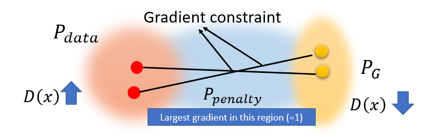
• In practical, the penalty is set as L2-norm, which constrain the largest gradient to 1
  • Overly large gradients penalty works but too small gradient will also cause gradient vanishing, which will slow down the convergence.

\[\begin{aligned} V(G, D) & \approx \max _{D} \{E_{x \sim P_{\text {data}}}[D(x)]-E_{x \sim P_{G}}[D(x)] -\lambda E_{x \sim P_{\text {penalty}}} [\max _{x}\left(0,\left\|\nabla_{x} D(x)\right\|-1\right)] \} \\ & \approx \max _{D} \{E_{x \sim P_{\text {data}}}[D(x)]-E_{x \sim P_{G}}[D(x)] -\lambda E_{x \sim P_{\text {penalty}}} [(\left\|\nabla_{x} D(x)\right\|-1 )^{2}] \} \end{aligned}\]

• Now discriminator will replace the last layer of the sigmoid function with wasserstain function to measure the distance between distributions, transmitting the problem from the binary classification to regression.

*reference-5

Spectrum Normalization

• Spectral Norm: keep the gradient norm smaller than 1 everywhere.
• We keep Lipschitz continuity for the weight $W$ of each layer of the neural network $f(x) = Wx$.
  • Each matrix of $W$ divide by the sigular value of itself will guarantee 1-Lipschitz continuity.

TODO: paper, https://blog.csdn.net/c9Yv2cf9I06K2A9E/article/details/87220341

*reference-6

Other Improvement

EBGAN

• Energy-based GAN (EBGAN): the same generator but the discriminator is with an auto-encoder framework.
  • EBGAN outputs the reconstruction image and get the reconstruction error to the input of the discriminator.
  • The error is the energy to determine the goodness of the generated result. The energy takes low values when it is the correct label and higher values for incorrect label.

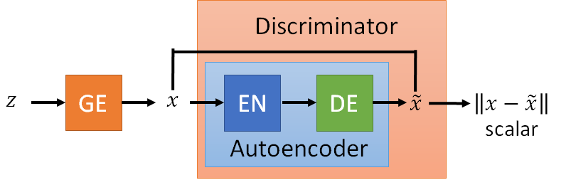
• Benefit: The auto-encoder discriminator can be pre-trained by real images without generator.
  • The discriminator can be expert at distinguish the real or fake at the beginning of the training the generator.
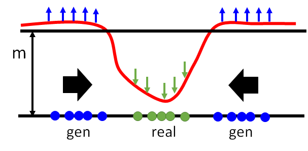
• \[\begin{aligned} &\mathcal{L}_{D}(x, z)=D(x)+\max (m-D(G(z))) \\ &\mathcal{L}_{G}(z)=D(G(z)) \end{aligned}\]
• For discriminators, to minimize $\mathcal{L}_{D}$ is to maximize $D(G(z))$, which means to raise the following curve in blue region.
• For generators, it makes effort to generate results with low energy.
• Without constraint, the curve will be lifted without limitation.
  • It is easy for the discriminator to increase the energy of fake result, lifting the curve, but hard for the generator to decrease the energy.
  • Set the margain to constrain the energy lifted by the discriminator.

TODO paper read https://blog.csdn.net/a312863063/article/details/88125429

*reference-8

Loss-sensitive GAN

TODO paper read

BE GAN

TODO paper read https://www.cnblogs.com/king-lps/p/8552177.html

Improved Algorithm

• Comparing to the original version of GAN algorithm:
  • Replace the log divergence with Wasserstein Distance.
  • Add Weight Clipping and Gradient Penalty.
• In each training iteration:
  • Learning D: find lower bound of $\max_D V(G,D)$ and repeat k times for fully trained.
    • Sample m examples $\{ x^{1}, x^{2}, \ldots, x^{m} \}$ from database distribution $P_{data}(x)$.
    • Sample m noise samples $\{z^{1}, z^{2}, \ldots, z^{m}\}$ from the prior $P_{prior}(z)$.
    • Obtaining generated data $\{\tilde{x}^{1}, \tilde{x}^{2}, \ldots, \tilde{x}^{m}\}, \tilde{x}^{i}=G\left(z^{i}\right), \tilde{x}^i = G(z^i)$.
    • Update discriminator paramters $\theta_{d}$ to maximize.
      \(\begin{aligned} &\tilde{V}=\frac{1}{m} \sum_{i=1}^{m} \color{red}{D\left(x^{i}\right)-}\frac{1}{m} \sum_{i=1}^{m} \color{red}{D\left(\tilde{x}^{i}\right) } \\ &\theta_{d} \leftarrow \theta_{d}\color{red}{+}\eta \nabla \tilde{V}\left(\theta_{d}\right) \end{aligned}\)
  • Learning G: find the minimum of $\min_G V(G,D)$ only once.
  • Sample another m noise samples $\{z^{1}, z^{2}, \ldots, z^{m}\}$ from the prior $P_{prior}(z)$.
  • Update generator parameters $\theta_{g}$ to maximize
    \(\begin{aligned} &\tilde{V}= \color{red}{-} \frac{1}{m} \sum_{i=1}^{m} \color{red}{D(G\left(z^{i}\right))} \\ &\theta_{g} \leftarrow \theta_{g}\color{red}{-}\eta \nabla \tilde{V}\left(\theta_{g}\right) \end{aligned}\)

TODO: update $\tilde{V}$ with gradient penalty, check code.

Reference

1. Machine Learning And Having It Deep And Structured 2018 Spring, Hung-yi Lee
2. fGAN: General Framework of GAN
3. Wasserstein GAN and the Kantorovich-Rubinstein Duality
4. Wasserstein GAN
5. Improved Training of Wasserstein GANs
6. Spectral Normalization for Generative Adversarial Networks
7. Spectral Norm Explaination
8. Energy-based Generative Adversarial Network