Sequence Generation, Generation Evaluation, Inception Score, Fréchet Inception Distance
Sequence to Sequence
-
The generator is a typical seq2seq model.
- Conditional Squence Generation
- Reinforcement Learning (human feedback)
- GAN (discriminator feedback)
- Unsupervised Conditional Sequence Generation
- Text style transfer
- Unsupervised Abstractive Summarization
- Unsupervised Translation
- The problem of seq2seq: the result by maximizing likelihood satisfying the training criterion, but contracting the human sense
- For the chat-bot:
I'm goodis similar toI'am XXXbut is not the answer toHow are you?.
- For the chat-bot:
Reinforcement Learning
- Input sentence $h$, through Chatbot $En$ and $De$, output response sentence $x$.
- Learn to maximize expected reward by policy gradient.
- Input sentence $h$ and response sentece $x$, through human, output the reward $R(h,x)$.
- Behave as a discriminator.
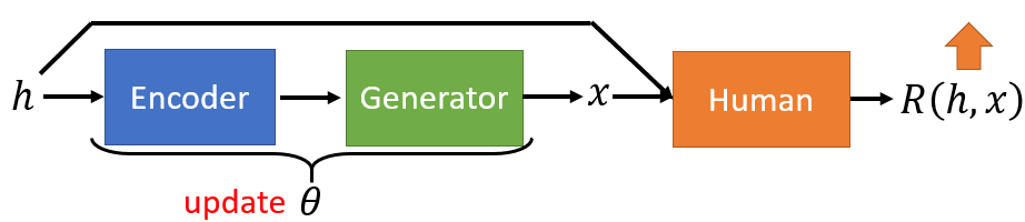
- Target: to find the optimal $\theta$ to maximize the expected reward.
- Accumulate over the distribution of input sentence $h$, and over all possibility of output $x$ caused by the randomness in generator.
- Accumulation of the possiblity is computing the expectation.
- Approximate the real expectation by sampling as much as possible.
- Sampling approximate the target reward, but $R(h^i,x^i)$ is unrelated to the parameter $\theta$ of the network.
- Now $R$ is related to parameter $\theta$,
- Update $\theta$ regarding to the reward:
$ \theta^{\textit{new}} \leftarrow \theta^{\textit{old}} + \eta \nabla \bar{R}_{\theta^{\textit{old}}} $
- When $R\left(h^{i}, x^{i}\right) $ is positive, $P_{\theta}(x^i \mid h^i)$ will increase.
- When $R\left(h^{i}, x^{i}\right) $ is negative, $P_{\theta}(x^i \mid h^i)$ will decrease.
- After each iteration of updating $\theta$, it is necessary to do sampling again before computing the gradient.
- Because the reward $\bar{R}_{\theta}$ will change after each update operations of $\theta$.
- Comparing Reinforcement Learning with Maximize Likelihood:
- Maximum Likelihood is identical to minimize cross entropy.
- Train the model based on supervised learning using paired data.
- Gradient descent on tje pnkect function.
- Reinforcement learning is kind of weighted objective function of maximum likelihood.
- RL obtained the training data from the interaction during the training process.
- Derive the objective function from the gradient equation, analogy with maximum likelihood.
- Maximum Likelihood is identical to minimize cross entropy.
| Maximum Likelihood | Reinforcement Learning | |
|---|---|---|
| Objective Function | \(\frac{1}{N} \sum_{i=1}^{N} \log P_{\theta}\left(\hat{x}^{i} \mid c^{i}\right)\) | \(\frac{1}{N} \sum_{i=1}^{N} R\left(c^{i}, x^{i}\right) \log P_{\theta}\left(x^{i} \mid c^{i}\right)\) |
| Gradient | \(\frac{1}{N} \sum_{i=1}^{N} \nabla \log P_{\theta}\left(\hat{x}^{i} \mid c^{i}\right)\) | \(\frac{1}{N} \sum_{i=1}^{N} R\left(c^{i}, x^{i}\right) \nabla \log P_{\theta}\left(x^{i} \mid c^{i}\right)\) |
| Training Data | \(\left\{\left(c^{1}, \hat{x}^{1}\right), \ldots,\left(c^{N}, \hat{x}^{N}\right)\right\} \\ R\left(c^{i}, \hat{x}^{i}\right)=1\) | \(\left\{\left(c^{1}, x^{1}\right), \ldots,\left(c^{N}, x^{N}\right)\right\}\) obtained from interation, weighted by $R(c^i, x^i)$ |
Conditional GAN
- Similar to Reinforcement Learning
- Input sentence $h$, through Chatbot $En$ and $De$, output response sentence $x$.
- Learn to maximize expected reward by policy gradient.
- Replace Human with discriminator
- Input sentence $h$ and response sentece $x$, through discriminator, output real or fake (reward).
- Input human dialogues, through discriminator, output real or fake (reward).
Warning: Sometimes discriminator may immediately distinguish the fake one-hot score, because comparing to the true label where the only exact true dimension contains 1, fake score vector is diffused as [0.8, 0.1, 0, ..., 0.1]. Thus, WGAN solves this problem by constraining the discriminator with 1-Lipschitz function, whereby the discriminator’s vision becomes ‘fuzzy’ and scores are not distinguished too much.
Evaluation
- Evaluate the quality of the generation from GAN
Likelihood
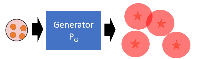
- The traditional method is to measure the likelihood of the generation of the well-trained GAN $P_G$.
- Compare the likelihood with the real data distribution.
- If it has the higher possibility of $P_G$ to generate the real data, we assume $P_G$ is better.
- The problem is there is no way to compute the generation distribution $P_G(x^i)$.
- Because the data is generated according to the prior distribution. The amount of the output is limited and the content is not determinated.
- Kernel Density Estimation: estimate the distribution $P_G(x)$ from sampling, and assume the generated result is Guassian Mixture Model (GMM) to approximate $P_G$.
- Each generated sample is the mean of a Gaussian with the same covariance.
- The problem still exists:
- The number of sampling is uncertain which is enough to make sure the accuracy of GMM.
- GMM is too naive to represent a complicated generator.
- Likelihood can not represent the quality of results.
Note: Likelihood only gives the similarity of the generation to the real data, but has no indication on the quality of the generated result which is not in the dataset. Also, likelihood doesn’t guarantee the diversity of the generation.
Objective Evaluation
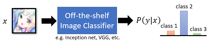
- Train an image classifier to evaluate the generator good or not.
- Intuitively, if the well-trained classifier recognize the image and give the clear category to the result, the generation is generally not bad.
- If we have the generated image $x$ and the output $y$ from the classifier evaluator,
- For the quality of the generation, more concentrated distribution means the higher visual quality.
- For the diversity of the generation, the more uniform distribution of all generated outputs means the higher diversity.
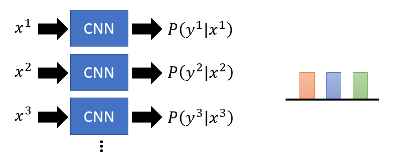
- For the quality of the generation, more concentrated distribution means the higher visual quality.
Inception Score
- A well-trained inception network (Inception Net-V3) as a classifier to evaluate the generation.
- Take the image as an input, output
1000dimensional vector, where each dimension represents the possibility of one class. - The whole vector represents the possibility distribution.
- Take the image as an input, output
- For each single generated image, the entropy of the possibility distribution from the Inception Net should be as small as possibile.
- The smaller entropy means the more confident on the classification result and the better quality of the image.
\(\begin{aligned} & E_{x \sim p_{G}}(H(p(y \mid x))) \\ =& \sum_{x \in G} P(x) H(p(y \mid x)) \\ =& -\sum_{x \in G} P(x) \sum_{i=1}^{1000} P\left(y_{i} \mid x\right) \log P\left(y_{i} \mid x\right) \\ \end{aligned}\)
- The smaller entropy means the more confident on the classification result and the better quality of the image.
- For the batch of generated image, the entropy of the average possibility distribution should be as large as possibile.
- To ensure the diversity of generated images, the possibility distribution over different images should vary a lot.
- Larger divergence makes the total distribution more prone to the uniform distribution, and the larger entropy.
\(\begin{aligned} & H\left(E_{x \sim p_{G}}(p(y \mid x))\right) \\ =& H\left(\sum_{x \in G} P(x) p(y \mid x)\right) \\ =& H(p(y)) \\ =& -\sum_{i=1}^{1000} P\left(y_{i}\right) \log P\left(y_{i}\right) \\ =& -\sum_{i=1}^{1000} \sum_{x \in G} P\left(y_{i}, x\right) \log P\left(y_{i}\right) \\ =& -\sum_{x \in G} P(x) \sum_{i=1}^{1000} P\left(y_{i} \mid x\right) \log P\left(y_{i}\right) \end{aligned}\)
- Inception score combines the negative of the entropy of image quality and positive of the entropy of image diversity, and take exponential.
- Inception score is the
KL-divergenceof $p(y|x)$ and $p(y)$.
- Inception score is the
- In practical, we generate ${x_1,x_2,…,x_n}$ from the generator and compute $P(y_i)$ first and then compute IS by
In summary: The higher Inception Score (IS) means the better quality and diversity.
Fréchet Inception Distance
- Fréchet Inception Distance (FID): similar to Inception Score, based on Inception Net-V3.
- Comparing to IS which evaluate directly on the generated images distribution, FID make comparison between generated images and real images and calculate distances.
- Assume the generated images is subject to a certain type of distribution, if the generated distribution and real distribution are closed, the generation is reasonable.
-
$\mu,\Sigma$ represents the mean and covariance matrix in real image $x$ and generated set $g$, $\text{Tr}$ is the trace of the matrix.
-
The covariance matrix is as large as the size of
pixel*pixeldimensions and spatial expensive.- Thus, replace the last layer of Inception Network with a layer of
2048dimensional predictor output size.
- Thus, replace the last layer of Inception Network with a layer of
In summary: The lower Fréchet Inception Distance (FID) means the the real distribution are more closed to the real images. The better real image set and the lower FID means the better generation,
Other Problems
- Even the generated result is high quality and clear, it still cannot ensure the good generator.
- GAN is inclined to memory the image in dataset with minor modification.
- The picture shifted several pixels is closed to the original version in Enclidean Distance, but the same amount of distance can produce totally different image with different semantic category.
- In other words, if the generated image is the shifted version of one in dataset, the generator may be rated as good due to the Enclidean similarity, but the diversity is still bad.
TODO DCGAN
TODO ALI