The Notes of Computer Graphics Ⅳ

Rasterization, Sampling, Frequency and Filtering, Antialiasing, Z-buffer

After Viewing transformation

• Viewport transformation: project the canonical cube $\left[-1, 1\right]^3$, we get from viewing transformation, to the screen.

Screen

• An array of pixels
• Size of the array: resolution (i.e. 1920 x 1080)
• A typical kind of raster display

Raster

• Raster == screen in German
• Rasterize – drawing onto the screen

Pixel

• short for picture element
• For now: A pixel is a little square with uniform color. Actually not in actual electronic display.
• Color is a mixture of (red, green, blue)

For the real displays of LCD screen. Each pixel is not uniform color, but R,G,B pixel geometry. Even so, now we assume a colored square full-color pixel.

Info: Bayer Pattern(Filter) is shown on the right, where green elements are twice as many as red or blue to mimic the physiology of the human eye which is more sensitive to green light.

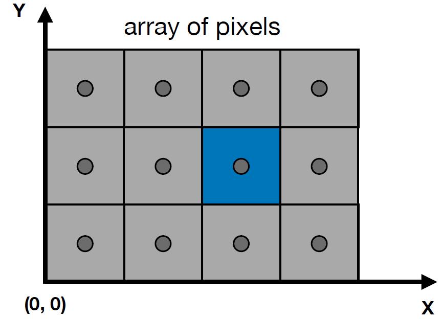
Screen space

• Following definition is slightly different from tiger book

  • Pixels indices are in the form of $(x,y)$, where both $x$ and $y$ are integers
  • Pixels indices are from $(0,0)$ to $(width-1, height-1)$
  • Pixel $(x,y)$ is centered at $(x+0.5, y+0.5)$
  • The screen covers range $(0,0)$ to $(width, height)$

Canonical Cube to Screen

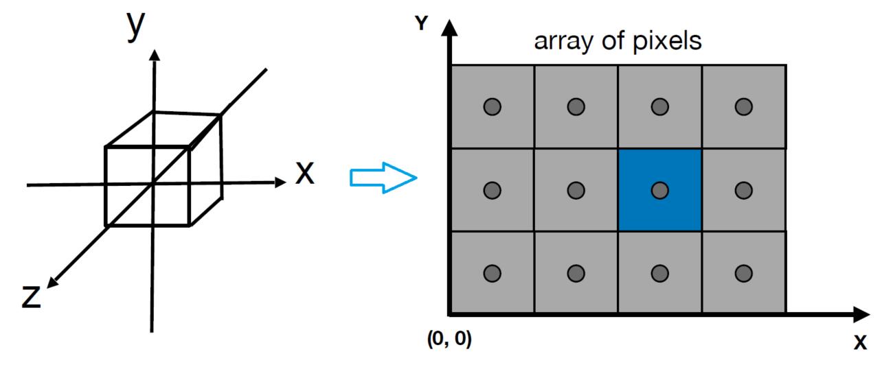
• irrelevant to $z$
• Transform in $xy$ plane: $\left[-1, 1\right]^2$ to $\left[0, width\right]^2 \times \left[0, height\right]^2$
• Viewport transform matrix

Raster Displays

• CRT (Cathode Ray Tube)
• Television: Raster Display CRT
• In fact, pixel, the component geometry in an image sensor or display, has three primary color: red, blue and green, which can be ordered in different patterns

Tip: On the memory of PC or Graphic Processing Unit (GPU), Frame Buffer is the memory for a raster display.

• LCD (Liquid Crystal Display)
  • Principle: block or transmit light by twisting polarization(极化, 偏振方向)
  • Base on the wave property of light
• Electrophoretic

Rasterization

Rasterization: Drawing to Raster Display

Triangles = Fundamental Shape

• Most basic polygon
  • break up other polygons
• Unique properties
  • Guaranteed to be planar
  • Well-defined interior (How about the polygon which has holes in it, and how about concave polygons?)
  • Well-defined method for interpolating values at vertices over triangle (barycentric interpolation)

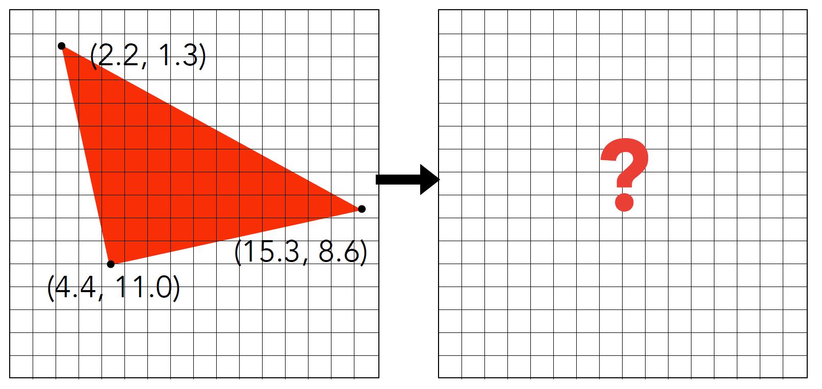
From Triangle to pixels

• Input: position of traingle vertices projected on screen
• Output: set of pixel values approximating triangle

Sampling a Function

• Evaluating a function at a point is sampling, we can discretize a function by sampling

Info: Sampling is a core idea in graphics. i.e. We sample time(1D), area (2D), direction (2D), volumn (3D). Here, the centers of pixels are used to sample screen space.

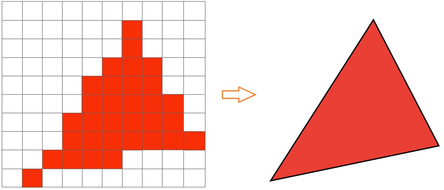
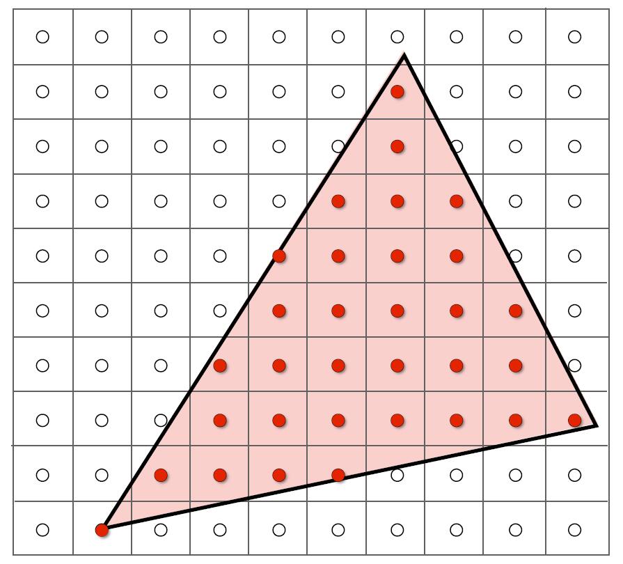
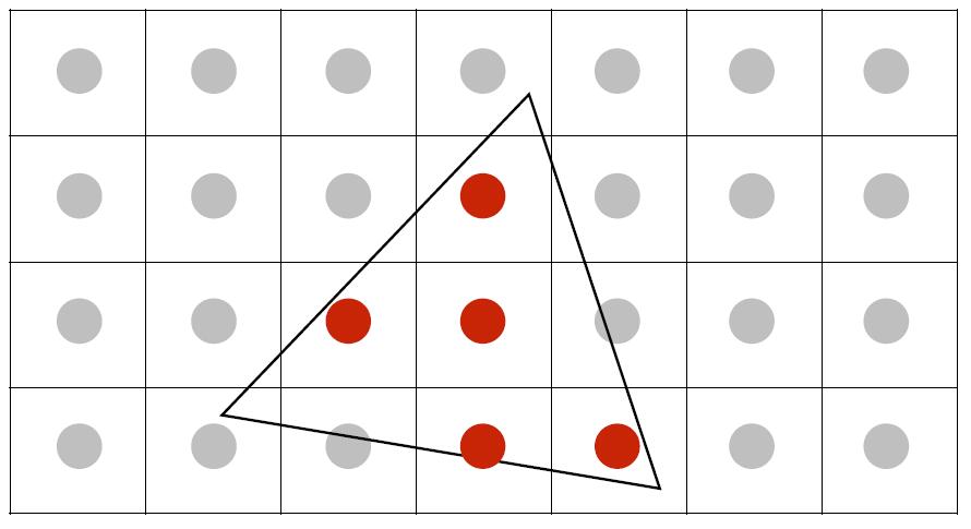
Rasterization as 2D Sampling

• Sample if each pixel center is inside triangle

bool inside(t, x, y) { // x, y: not necessarily integers
    if Point (x, y) in triangle t:
        return 1;
    return 0;
}

for (int x = 0; x < xmax; ++x)
    for (int y = 0; y < ymax; ++y)
        image[x][y] = inside(tri, x + 0.5, y + 0.5);

• Use three cross product to check if the Point is inside the triangle or not.
• Disregard edge cases when the sample point is exactly on the edge of the triangle.

Tip: Pixel values are integers so the center should be additional 0.5 amount.

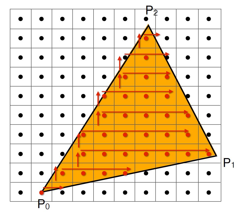
• Use Bounding Box (axis aligned) to avoid checking all pixels on the screen and reduce great time consumption.

• Incremental triangle traversal: traverse from the beginning of the left side of the triangle to the right.
  • Suitable for thin and rotated triangles, especially for those which has small area but consume the large proportion of bounding box

Sampling

Ubiquitous Sampling

• Rasterization = Sample 2D Positions
• Photograph = Sample Image Sensor Plane
• Video = Sample Time

Artifacts

• Artifacts: Errors, Mistakes, Inaccuracies

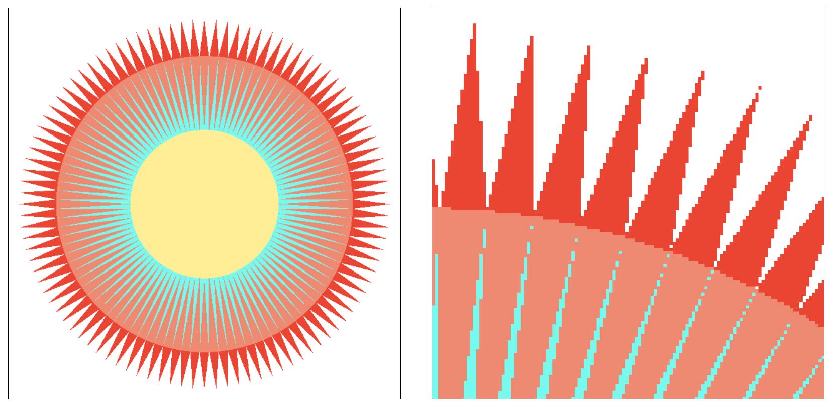
• Aliasing Artifacts due to sampling

  • Jaggies: sampling in space
  • Moire pattern: undersampling (skip odd rows and columns) images
  • Wagon wheel effect: sampling in time of our eyes

The reason behind the Aliasing Artifact

• Signals are changing too fast (high frequency) but sampled too slowly

Frequency and Filtering

• Central Idea: Blurring (pre-filtering) before sampling

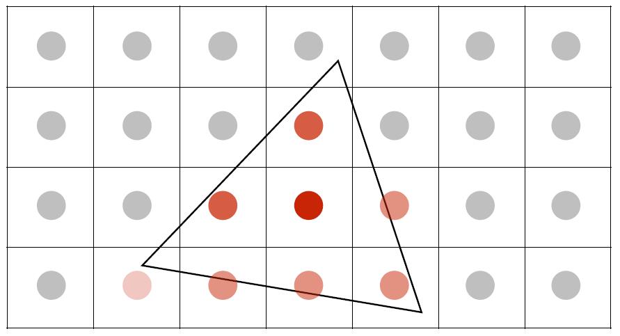
• Directly sample: pixel values of jaggies in rasterized triangle are pure red or white

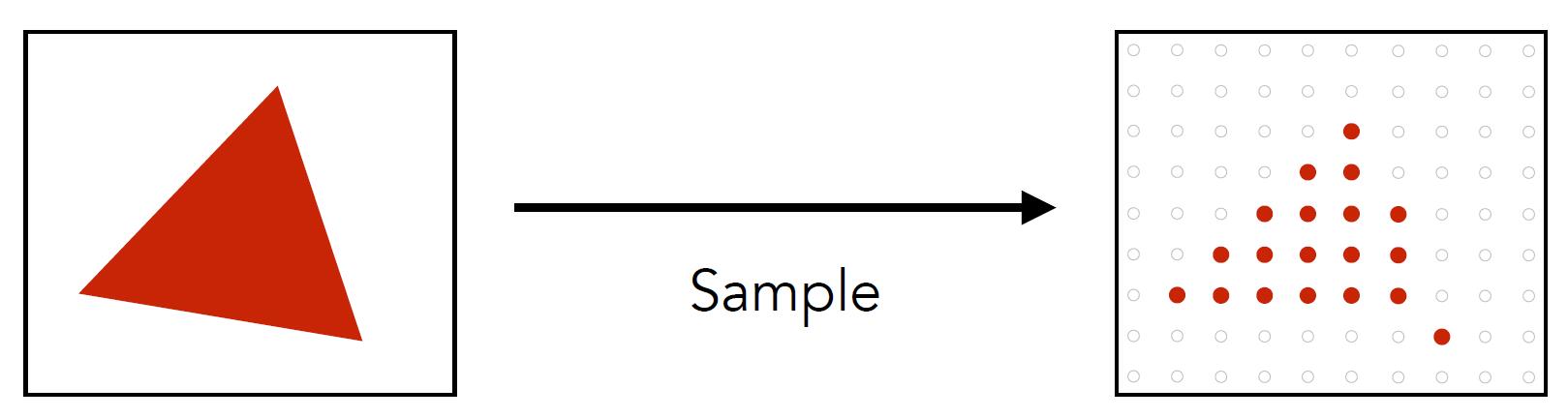
• Pre-filter before sample: pixel values of antialiased edges have intermediate values

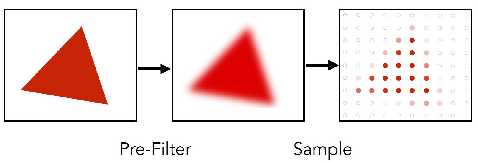
Tip: remove frequencies above Nyquist.

• The order of blurring and sampling matters

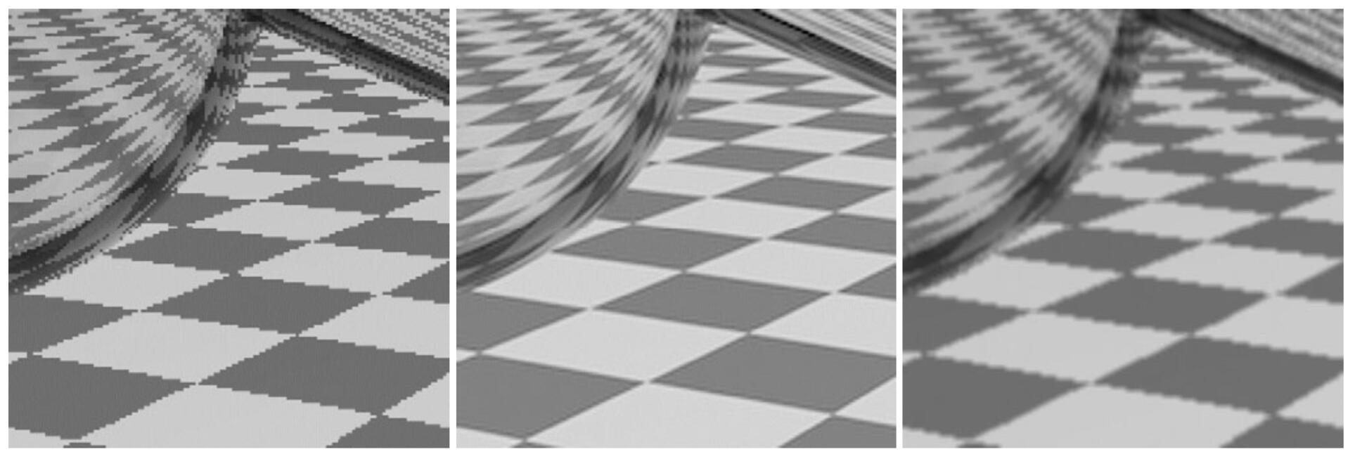
The above figures are sampling, antialiasing (filter then sample), blurred alisaing (sample then filter)

The reason why undersampling introduces aliasing, and prefiltering then sampling can do antialiasing instead of the inversed operation will be explained at Antialiasing.

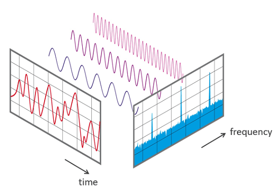
Fourier Transform

• Frequency: $f$ in $sin(2\pi fx)$, where $f = \frac{1}{T}$

• Represent a function as a weighted sum of sines and cosines.

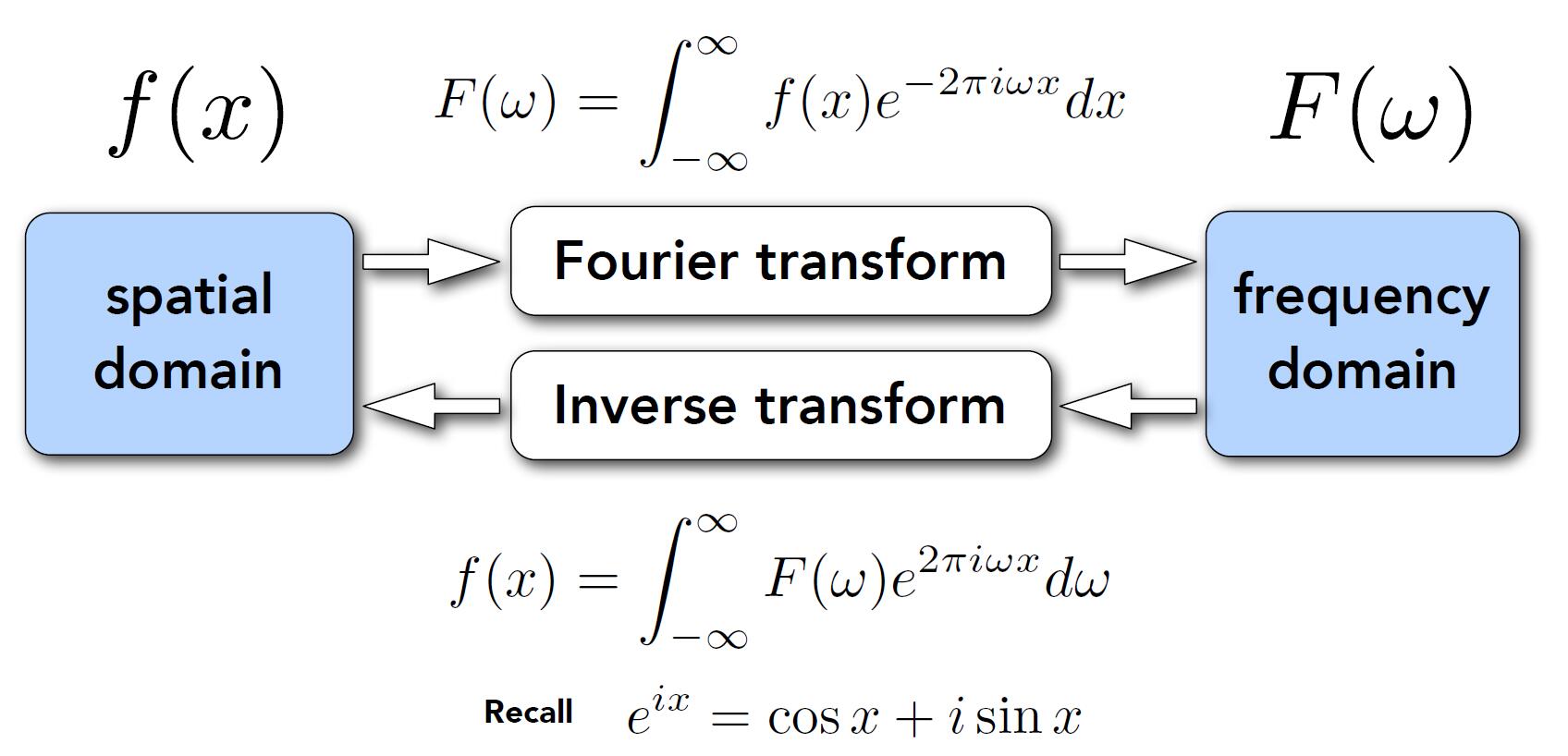
• Fourier transform decomposes a signal into frequencies, from spatial domain to frequency domain

Nyquist Theory

• Low frequency signal: sampled adequately for reasonable reconstruction
• High frequency signal: insufficiently sampled and reconstruction is correct

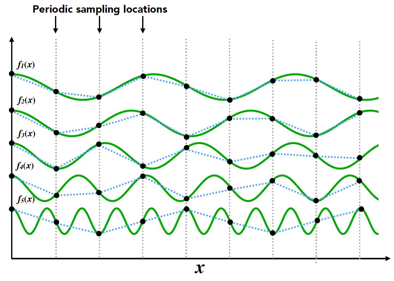
• Thus, higher frequencies need faster sampling
• Strictly, the sampling frequency should at least be twice the signal bandwidth. This frequency is called Nyquist rate

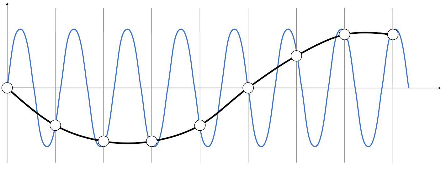
• Two frequencies (above blue and black) that are indistinguishable at a given sampling rate called aliases.

Filtering

Filtering: Getting rid of certain frequency contents

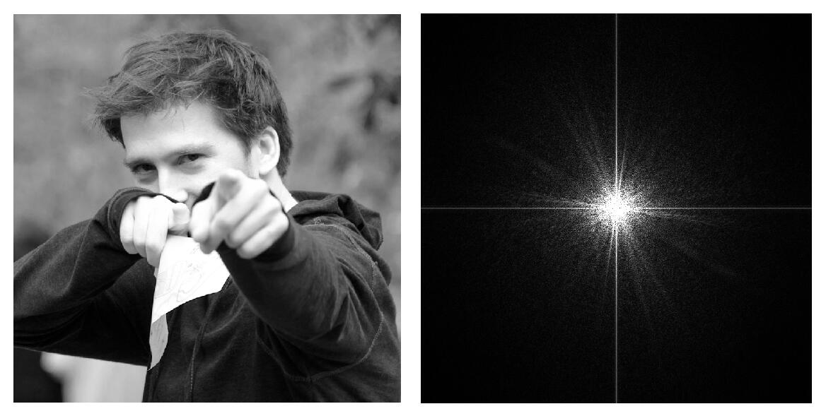
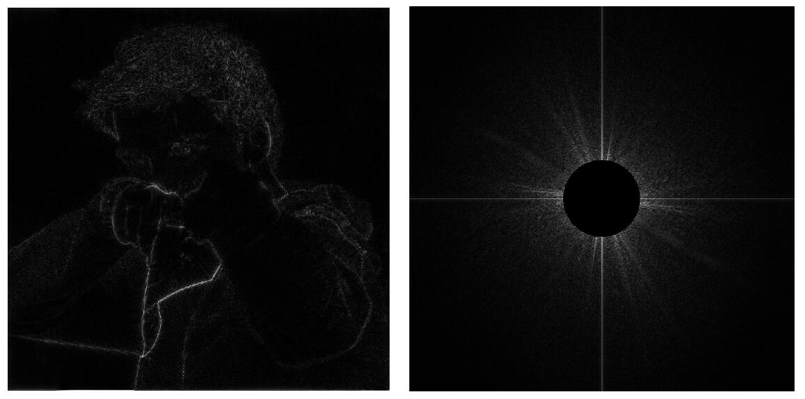
• The right image shows the value of frequency domain which is transformed by Fourier Transform from the left image, spatial domain.

• Above two-dimensional transform formula shows that the original image $f(x,y)$ is transformed into $F(u,v)$

• In the right figure, the center represents $u =0,v=0$, that is $F(0,0)$. This means the center of the image is the low frequency region, otherwise high frequency region.

• High-pass filter will get rid of all low frequency and keep edges of the image.

• Low-pass filter will filter the high frequency and retain the smooth part of the image.

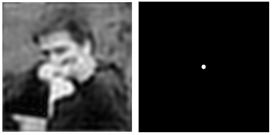
Tip: For the two-dimensional Fourier Transform, the image can be thought of as being tiled (stacked vertically and horizontally) infinitely. Thus two highlight strips in a cross shape at the center of the image is caused by the drastic change of the edges of the left figures.

Convolution

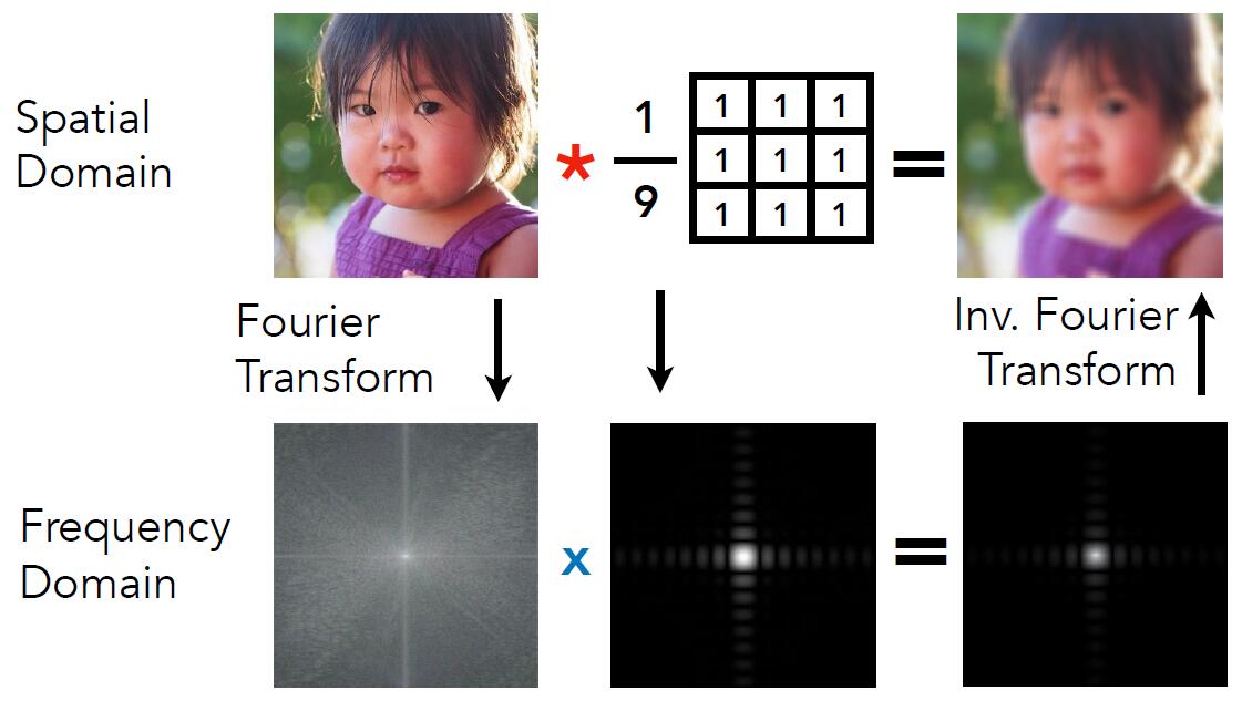
• Convolution in spatial domain is equivalent to multiplication in frequency domain, and vice versa

An intuitive proof: The spatial domain signal can be decomposed into a series of sinusoidal signals with different frequencies. According to the distributive property of convolution operation, the convolution of two spatial signals can be regarded as the sum of the convolutions of pairwise sinusoidal signals. Since the result of the convolution of sinusodial signals with different frequencies is zero, only the convolution of sinusoidal signals with the same frequency is left. As a result, the output of convolution is that the frequency remains unchanged and the amplitude is to be multiplied. For frequency domain, it appears as direct multiplication.

• Option 1:
  • Filter by convolution in the spatial domain
• Option 2:
  • Transform to frequency domain (Fourier transform)
  • Multiply by Fourier transform of convolution kernel
  • Transform back to spatial domain (inverse Fourier)

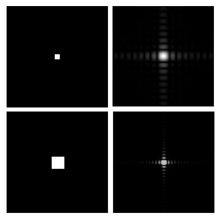
• Regularization term (i.e. $\frac{1}{9}$ in the above image) is to ensure the brightness of theimage does not change after transformation.

• Wider Filter Kernel = Lower Frequency

• Sampling = Repeating Frequency Contents

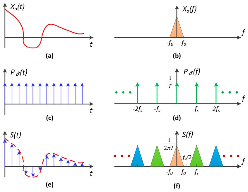
• (a) band-unlimited signal
• (b) frequency spectrum of (a)
• (c) unit-impulse function, which is used to simulate sampling
• (d) frequency spectrum of (b)
• (e) result of convolution of (a) and (c)

• (f) result of multiplication of (d) and (f). More intuitive, (f) is copied for many times along the frequency axis.

• Aliasing = Mixed Frequency Contents

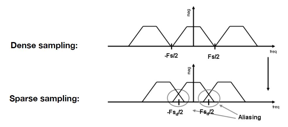
• When the sampling interval becomes small, the corresponding sampling frequency will become relatively large, which will lead to the overlapping phenomenon in final frequency spectrum. Thus, aliasing is caused by information lost.

Antialiasing

Basic theory

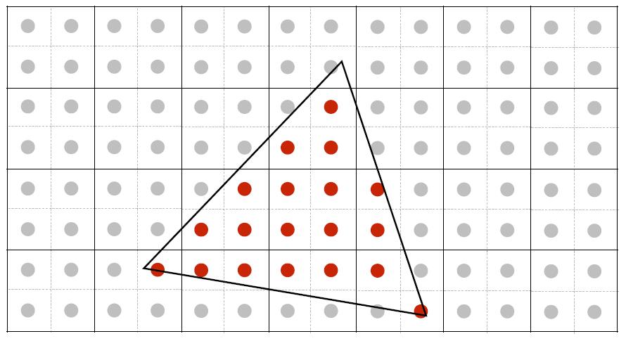
• Option 1: Increase sampling rate
  • Eseentially increasing the distance between replicas in the Fourier domain
  • Higher resolution displays, sensors, framebuffers..
  • Disadvantage: costly & may need very high resolution
• Option 2: Antialiasing
  • Making Fourier contents “narrower” before repeating
  • i.e. Filtering out high frequencies before sampling

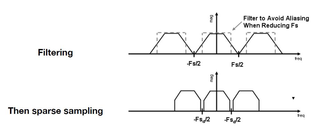
Perform filtering before the sampling will discard the high frequency and reduce the overlapping phenomenon, consequently reduce the loss of information and aliasing.

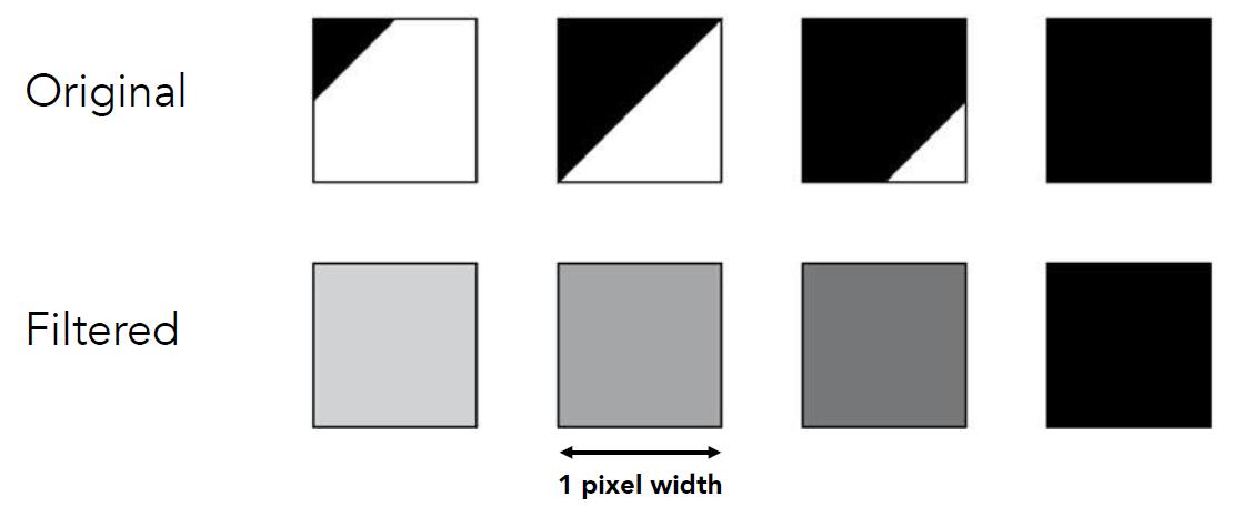
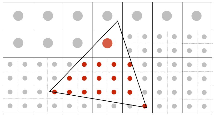
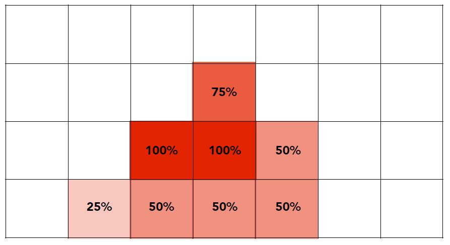
• Antialiasing by averaging values in pixel area
  • Convolve by a 1-pixel box-blur (convolving = filtering = averaing)
  • Sample at every pixel’s center
• In rasterizing one triangle, the average value inside a pixel area is equal to the area of the pixel covered by the triangle

• Sampling is an irreversable mapping, so the combination of convolution mapping and sampling is not commutative.

• Generally, antialiasing is to filter the high frequency signal so that the sampling frequency could catch up with the signal frequency.

MSAA

• MSAA (multi-sample antialiasing) is to antialias by supersampling: Approximate the effect of the 1-pixel box filter by sampling multiple locations within a pixel and averagin their values.
  • One sample per pixel
  • Take N x N samples in each pixel
  • Average the N x N samples inside each pixel
  • Until all pixel are averaged
  • Corresponding signal emitted by the display

Take 4 x MSAA as an example, given a screen with a resolution of 800 x 600, MSAA firstly render the image to the buffer of 1600 x 1200, and downsample it back to the original 800 x 600.

• The cost of MSAA is time consuming, the size of render target increases to the MSAA multiple times.

• The more multiplier of MSAA, the better performace of antialiasing, the more cost of time.

Milestones of Antialiasing

• FXAA (Fast Approximate AA): screen-space anti-aliasing algorithm. Different with MSAA which process the image before the sampling, FXAA postprocess the image after sampled and rasterized. FXAA contrast pixels to heuristically find edges and optimize jaggies in different directions. Very fast!

• TAA (Temporal AA) : reuse the previous frame and accordingly reduce the effects of temporal aliasing caused by the sampling rate of a scene being too low compared to the transformation speed of objects inside of the scene.

Tip: We often pronounce [temˈporəl] in industry to distinguish with ‘temporary’ meaning.

• Super resolution / super sampling
  • low resolution to high resolution
  • DLSS (Deep Learning Super Sampling): to understand and predict the missing information

Visibility and Occlusion

Painter’s Algorithm

• Solve the problem of triangles rendering order

• Inspired by how painters paint: Paint from back to front, overwrite in the framebuffer.

• Require sorting in depth $Olog(n)$ for n triangles

• unresolvable depth order exist:

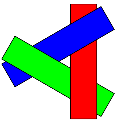
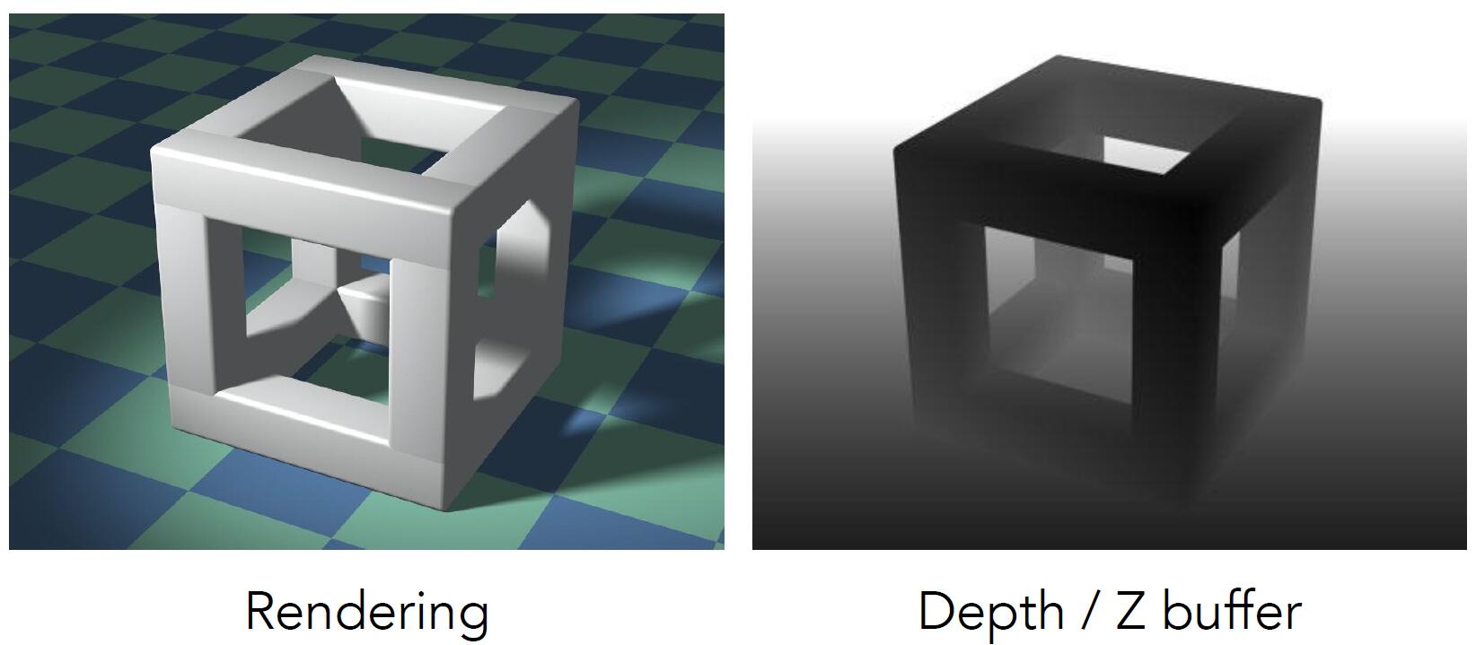
Z-Buffer

• store current minimum of z-value for each pixel
• need an additional buffer for depth values
  • frame buffer stores color values
  • depth buffer (z-buffer) stores depth

Note: For simplicity we suppose z is always positive (smaller z is closer, larger z is further)

Initialize depth buffer to +inf
// During rasterization
for each triangle T:
    for each sample(x, y, z) in T:
        if z < z_buffer[x, y]:  // closest sample so far
            frame_buffer[x, y] = rgb // update color
            z_buffer[x, y] = z  // update depth
        else
            pass // do nothing, this sample is occluded

• Complexity: $O(n)$ for traversing $n$ triangles
• Different order of drawing triangles has nothing to do with the result
• Most important visibility algorithm implemented in hardware for all GPUs

Tip: z-buffer can not deal with transparent objects.

Reference

• GAMES101, Lingqi Yan
• 图像傅里叶变换的频率
• 二维傅里叶变换
• FXAA、MSAA区别