Texture, Texture Mapping, Interpolation, Texture Filtering
Texture Mapping
- Texture mapping is to apply different colors at different places
- Texture defines property and color for each vertex
Surface
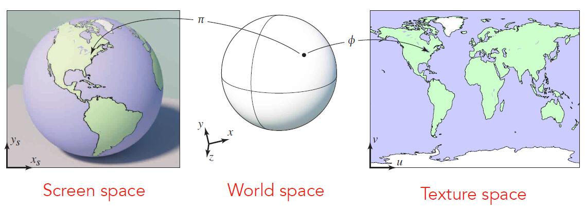
- Surfaces are 2D though lives in 3D world space
- Every 3D surface point also has a place where it goes in the 2D image (texture)
- In other words, each vertex of primitives in 3D world corresponds to the vertex of the primitive in 2D texture.
Texture
-
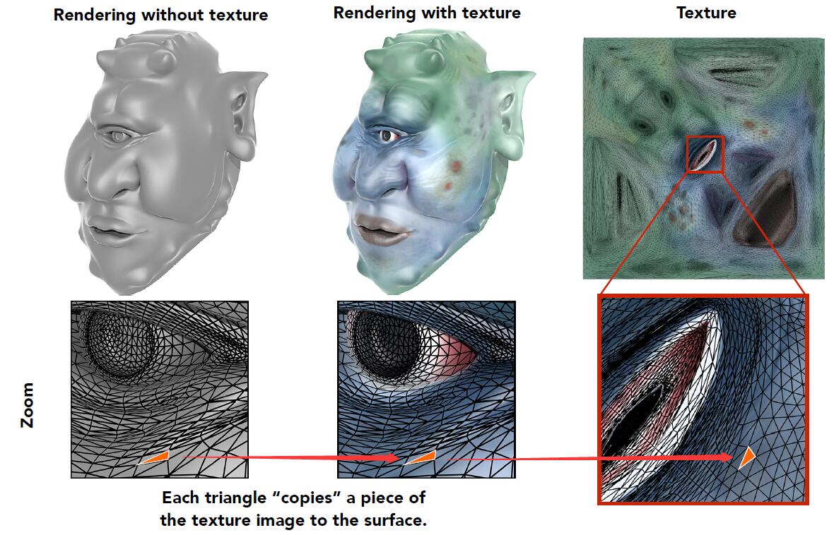
Texture is applied to Surface
-
We didn’t care about how mapping relationship of triangles produces between model and texture. The mapping and definition of primitives (triangles) are known.
- Generally, texture comes in two ways:
- Art designer design and produce the texture
- Parameterization of triangular meshes
- Parameterization is the process of finding parametric equations of a curve, a surface, a manifold or a variety, defined by an implicit equation.
Texture Coordinates
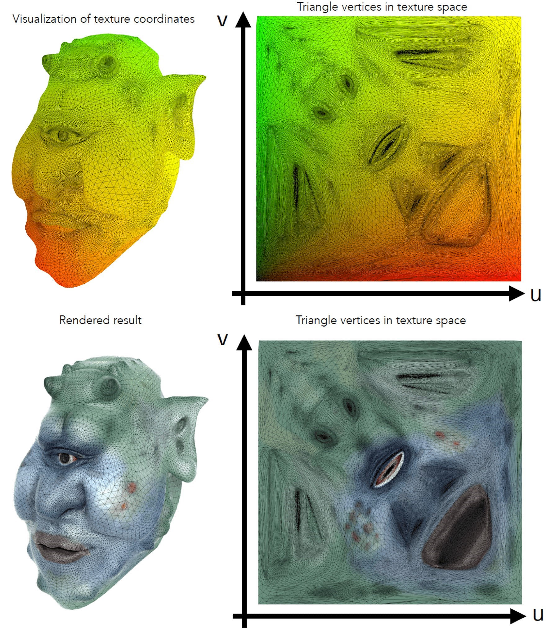
- Each triangle vertex is assigned a texture coordinate $(u,v)$.
- Define mapping between points on triangle’s surface (object coordinate space) to points in texture coordinate space.
- Each vertex corresponds to one texture mapping. Again, this mapping is known and we don’t care how this mapping come from.
Tip: No matter the texture is square or not, $u$ and $v$ are in range of $(0,1)$.
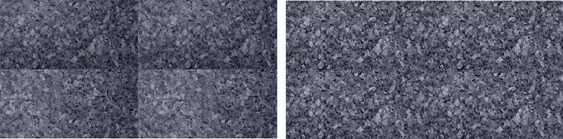
Texture Tile
- Textures can be applied multiple times
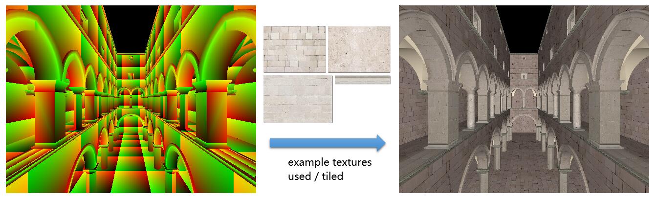
- Well-designed texture is tileable when multiple textures blend together profesionally and seamlessly together, borders of texture is not easily conspicuous.
Interpolation
Interpolation Across Triangles: Barycentric Coordinates
- Why to interpolate
- Specify values at vertices
- Obtain smoothly varying values across triangles
- What to interpolate
- Texture coordinates, colors, normal vectors. etc.
- How to interpolate
- Barycentric coordinate
Barycentric Coordinate
- Any point $(x,y)$ in the plane can be represented as a linear combination of triangular vertices.
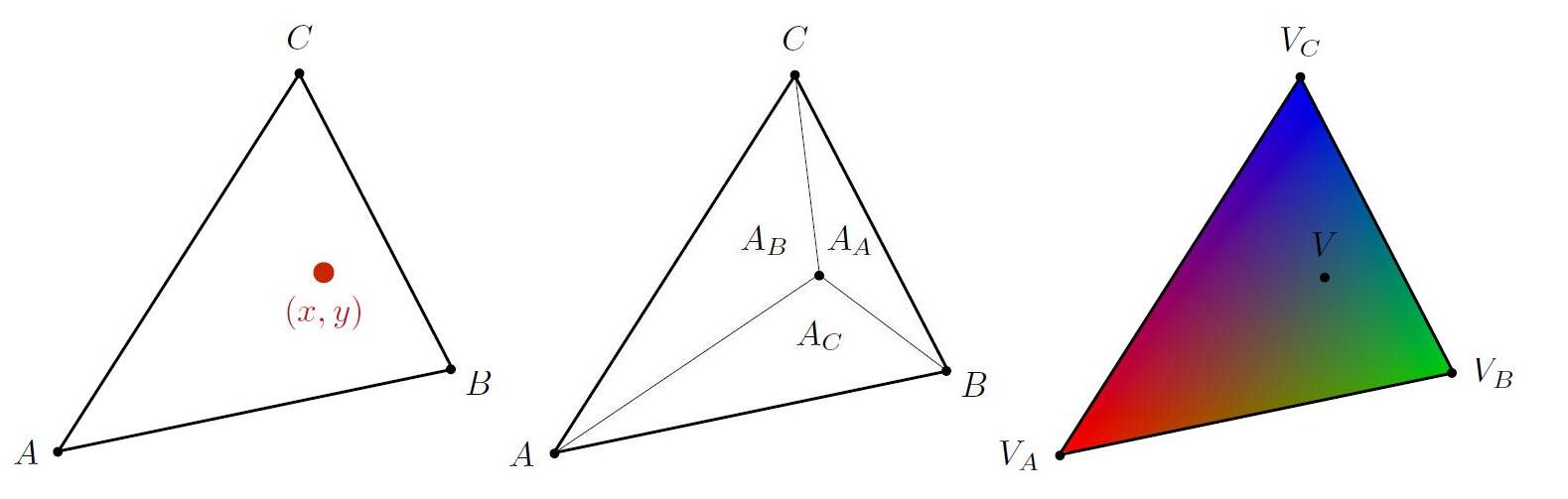
- A coordinate system for triangles $(\alpha, \beta, \gamma)$
- Proved by using point-scored formula
- Point $(x,y)$ is not in the plane of $ABC$ if $\alpha+\beta+\gamma \neq1$
- Point $(x,y)$ is inside the triangle if and only if all three $(\alpha, \beta, \gamma)$ are non-negative.
-
e.g. $A$ is when $(\alpha, \beta, \gamma) = (1, 0, 0)$
- Geometric viewpoint: proportional areas
- It is available to get $(\alpha, \beta, \gamma)$ by given a spcified point $(x,y)$.
-
Barycentric coordinate of centroid: $(\alpha, \beta, \gamma) = (\frac{1}{3}, \frac{1}{3}, \frac{1}{3})$, then $(x, y)=\frac{1}{3} A+\frac{1}{3} B+\frac{1}{3} C$
-
Linear interpolate values at vertices
- $V_A, V_B, V_C$ can be positions, texture coordinates, color, normal, depth, material attributes…
Note: barycentric coordinates are not invariant under projection! Thus interpolate every time after projections.
Texture Applying
- Simple texture mapping: diffuse color
for each rasterized screen sample (x, y):           // Usually a pixel's center
    (u, v) = evaluate texture coordinate at (x, y); // Using barycentric coordinates
    texcolor = texture.sample(u, v);                // get texture (u,v)
    set sample's color to texcolor;                 // Usually the diffuse albedo Kd of Blinn-Phong reflectance model
Texture Filtering
- To determine the texture color for a texture mapped pixel, using the colors near by texels.
- Texel (纹素): a pixel on a texture
- Two main categories of texture filtering, depending on the situation texture filtering
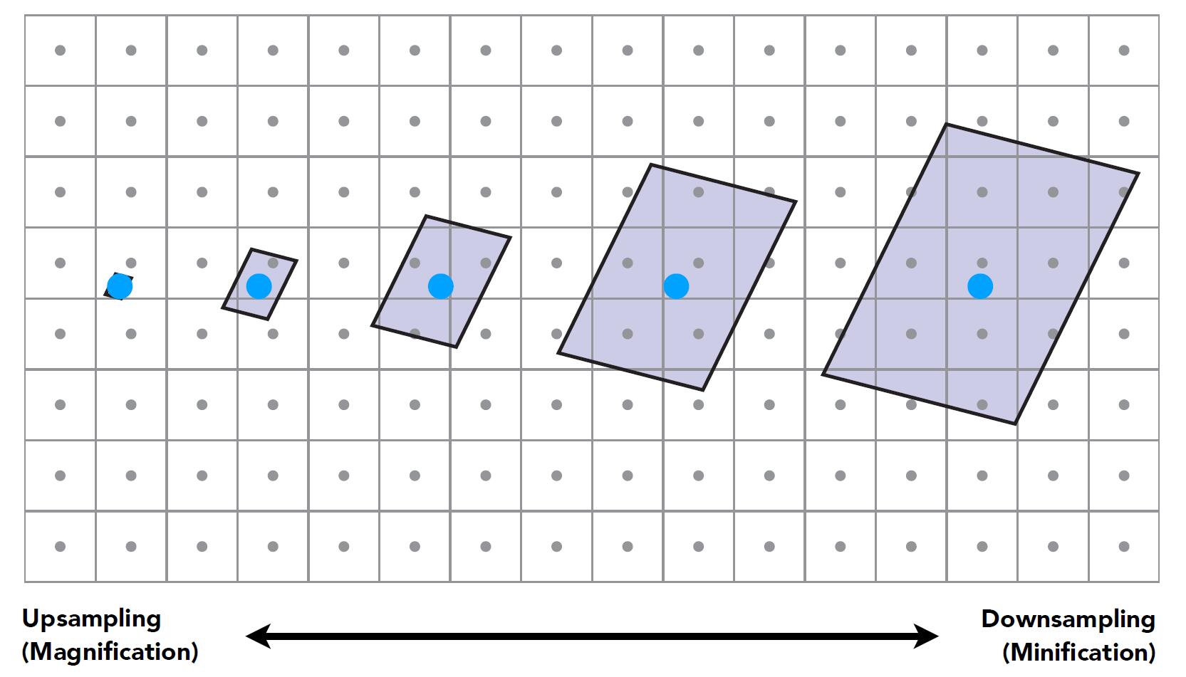
- Magnification filtering: a type of reconstruction filter where sparse data is interpolated to fill gaps
- Minification filtering: a type of anti-aliasing (AA), where texture samples exist at a higher frequency than required for the sample frequency needed for texture fill
Texture Magnification
- Insufficient texture resolution: texture is too small comparing to the object, then the texture has to be enlarged than its actual resolution.
Info: For each point on the object or scene, mapping it to the corresponding point on the low resolution texture will get non-integer coordinates of texture. Rounding off is the common process to obtain non-floating coordinate texel. As a result, multiple pixels of the object or scene will corresponds to the same texel of the texture, which means the generated figure is obscure of low quality. Thus interpolation handle it.
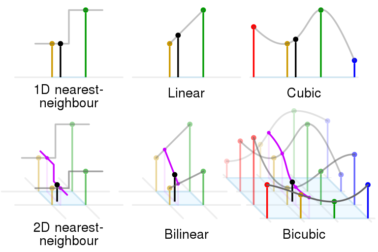
Bilinear Interpolation
- Linear interpolation (1D)
- Two horizontal interpolations
- Final vertical interpolation
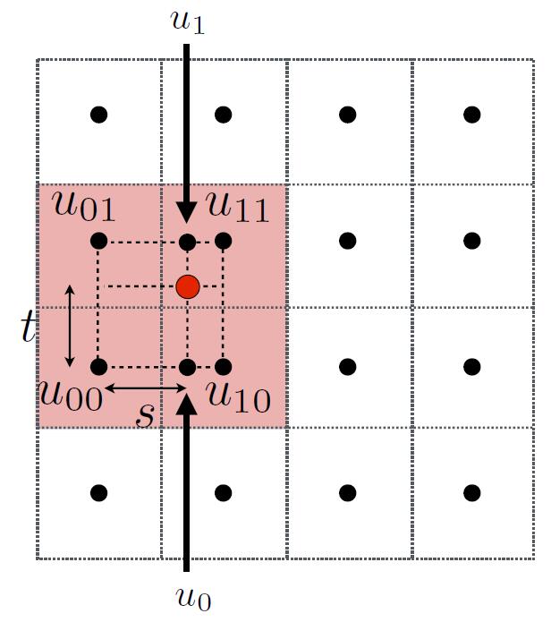
- Red point: want to sample texture value $f(x,y)$
-
Black points: indicate texture sample locations (the center of texel)
-
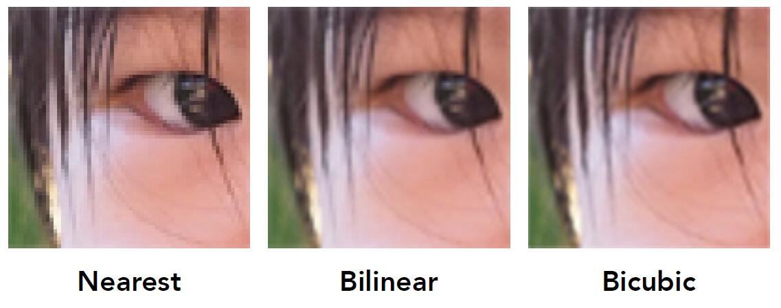
For the nearest method of texture applying, take the red point as an example, any mapping point in the square which the red point and $u_{11}$ locates at will take $u_{11}$ as a texel. When the object or scene is very large comparing to the texture, multiple pixels will map to the same texel as $u_{11}$. That is the reason why jaggies and artifacts are consipicuous in the above nearest figure.
-
For the bilinear interpolation, it takes 4 nearest sample locations with textrue values as labeled, blending the property and information of 4 texels, so the result is more smooth and realistic.
- Bilinear interpolation usually gives pretty good results at reasonable costs.
Bicubic Interpolation
- Bicubic interpolation is to use 4 x 4 point to do interpolation, which has better performance but higher costs. (Look into the canthus of the above figure, bilinear create jaggies but bicubic is more realistic)
Texture Minification
- Superadundant texture resolution: Texture is too large comparing to the screen space required, so it has to be shrunken relative to its natural resolution.
- Intuitively, when the texture is large, every information is available. But it is incorrect.
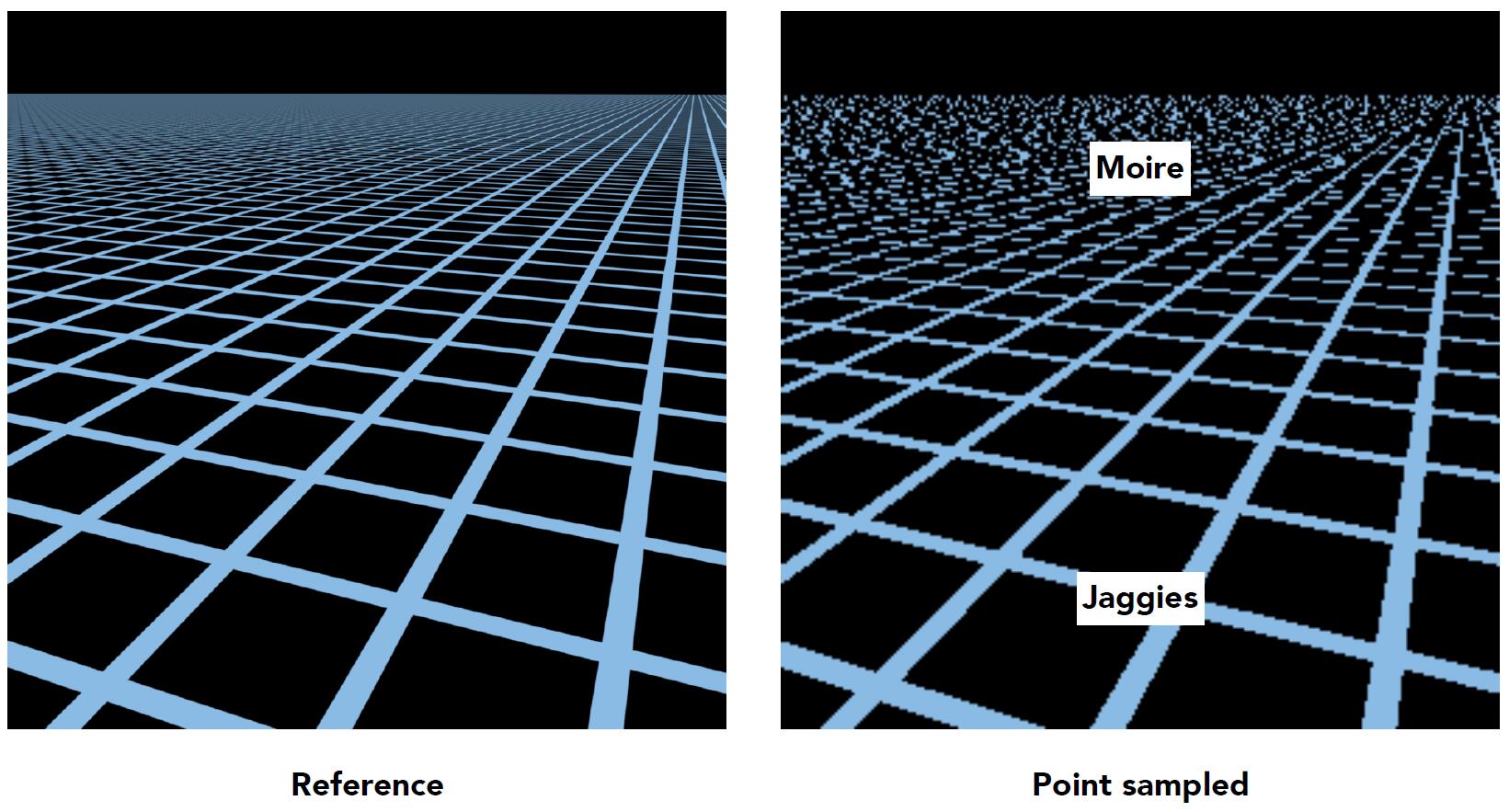
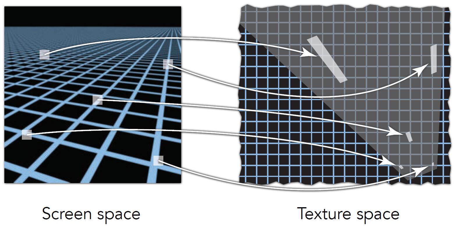
- Screen Pixel’s “Footprint” in Texture
- As the pixel in the screen space get growingly further, the number of corresponding texels in texture gets more and more.
- Take the above image as an example, the pixels close to the horizon represent a large region of texture. The information lost happens when the square which the blue point is inside is selected as texel
-
Supersampling to antialiasing: yes, high quality, but costly.
- The reason of aliasing when perform minification
- When highly minified, many texels in pixel footprint
- Signal frequency too large in a pixel
- Need even higher sampling frequency
- Solution: Not do sampling but get the average value within a range, Range Query.
Info: Some data structure like K-d tree, segment tree, binary indexed tree etc. are good ways to solve range query problem.
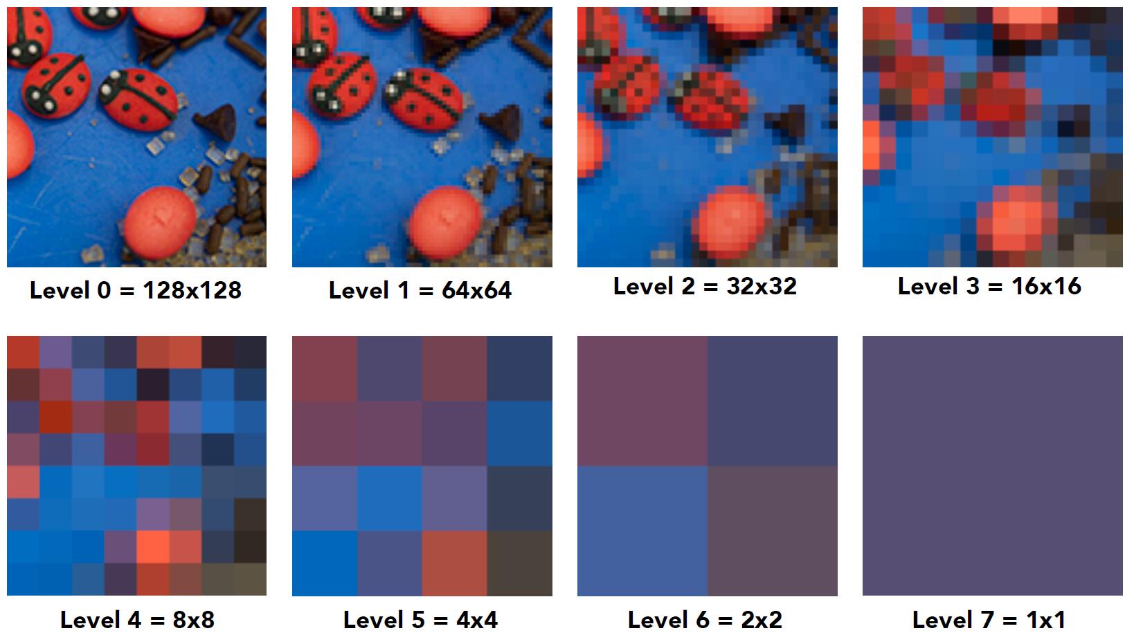
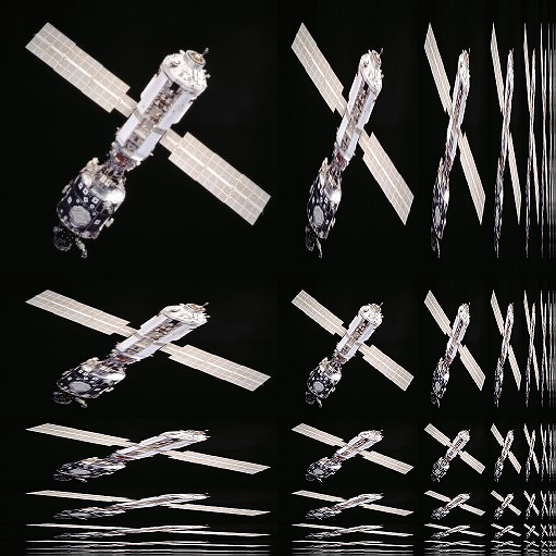
Mipmap
- Precompute and store the averages of the texture over various areas of different size and position.
- Allowing fast, approximate, square range queries.
- “Mip” comes from the Latin, meaning a multitude in a small space.
- A sequence of textures that contains the same image but at lower and lower resolution.
-
There are total of $log(n)$ images
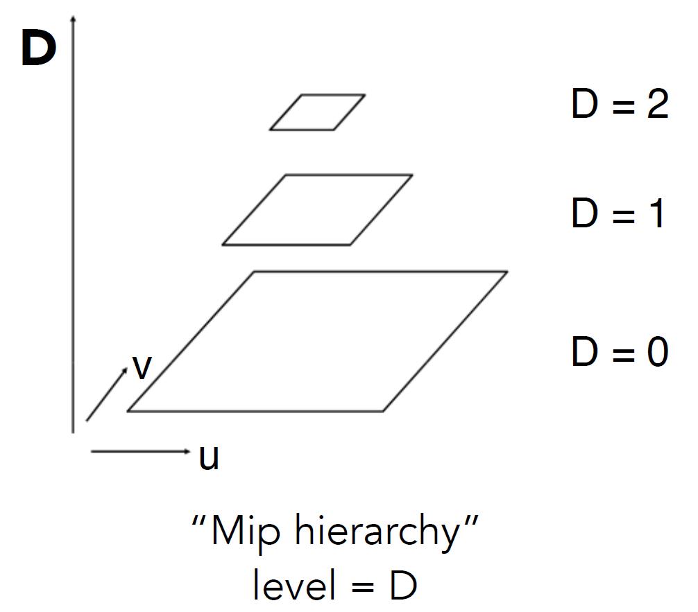
- The total storage overhead of a mipmap is the summation of series: $\frac{4}{3}$ to the original image.
Info: We call this kind of structure, with images that represent the same content at a series of lower and lower sampling rates, image pyramid in computer vision field.
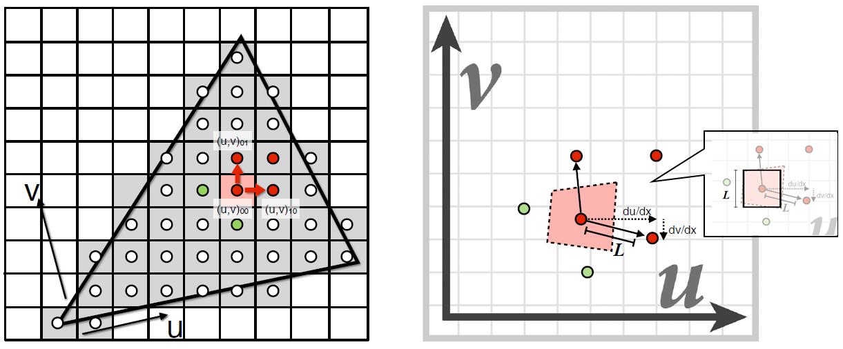
- Computing Mipmap at level $D$: estimate texture footprint using texture coordinates of neighboring screen samples
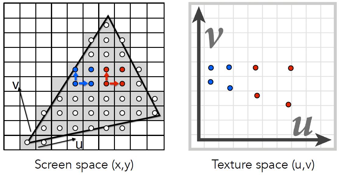
-
The distance between the pixel and neighbouring in screen space is 1
-
Denote the pixel $(x,y)$ in screen space and texel $(u,v)$ in texture space
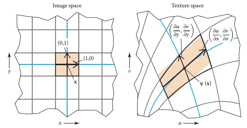
-
Denote transformation $\psi$ the mapping from image sapce to texture space as a linear mapping, the transformation equation, thus $u = \psi_{x}(x, y), v = \psi_{y}(x, y)$.
-
Jacobian matrix $J$ is the best linear approximation of $\psi$ in a neighbourhood of $(u,v)$ where $\psi$ is differentiable.
-
Recall that in linear transformation \(\left[\begin{array}{ll}a_{x} & b_{x} \\ a_{y} & b_{y}\end{array}\right]\left[\begin{array}{l}x \\ y\end{array}\right]=\left[\begin{array}{l}x^{\prime} \\ y^{\prime}\end{array}\right]\),\(\left[\begin{array}{ll}a_{x} & b_{x} \\ a_{y} & b_{y}\end{array}\right]\) is transformation matrix, the two columns of it \(\left[\begin{array}{l}a_{x} \\ a_{y}\end{array}\right]\) and \(\left[\begin{array}{l}a_{x} \\ a_{y}\end{array}\right]\) are two basis vector of the new space if the original basis is \(\left[\begin{array}{l}1 \\ 0\end{array}\right]\) and \(\left[\begin{array}{l}0 \\ 1\end{array}\right]\). Thus, we could take Jacobian matrix as transformation matrix mapping the pixel $(x, y)$ in screen space to the texture space $(u, v)$.
-
In screen space, suppose $(u, v)_{10}$ and $(u, v)_{01}$ as $(1, 0)$ and $(0, 1)$ relatively, the corresponding texel coordinate is computed by multiplying the transformation Jacobian matrix $J$:
Tip: Each column of Jacobian matrix is the new basis vector of the transformed space. More details
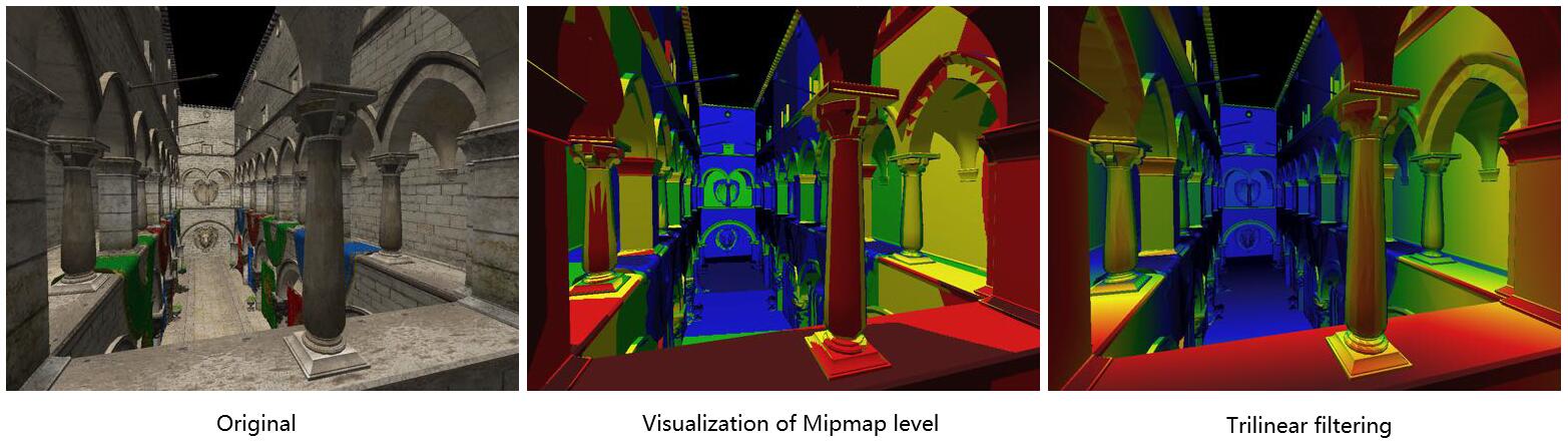
- Choose the level $D$ so that the size covered by the texels at that level is roughly the same as the overall size of the pixel footprint.
- $D$ rounded to nearest integer level
- near (in red) corresponds to low level of texture
- far (in blue) corresponds to high level of texture
-
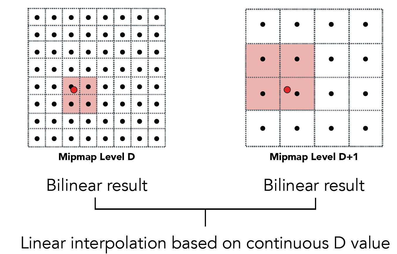
But Bilinear filtering only, where $D$ is clamped to nearest level, not support floating $D$ and the level $D$ is not continuous.
-
Trilinear Interpolation: perform two Bilinear interpolation in neighbouring levels and interpolate the interpolated result again.
Isotrpic Limitation
- Mipmap limitation
- the pixel footprint might be quite different in shape from the area represented by the texel, not always approximately square
- Mipmap is unable to handle the pixel footprint with an elongated shape
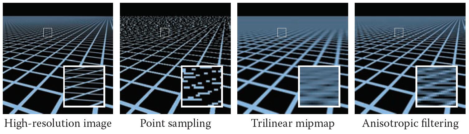
- Tilinear (isotropic) sampling will cause overblur problem most commonly when the points are on the floor that are far away viewed at very steep angles, which results in the pixel footprint covering much larger square areas.
- As a result, most footprints far from the viewer are averaged over the large area of the texture, which causes overblur.
Anisotropic filtering
- Anisotropic filtering(Ripmap, or abbreviated AF): use multiple lookups to approximate an elongated footprint better
- select the mipmap level based on the shortest axis of the footprint rather than the largest
- average together several lookups spaced along the long axis
- Look up axis-aligned rectangular zones and preserve detail at extreme viewing angles.
- Comparing to isotropic filtering which consume on third of extra space, anisotropic filtering takes three times of extra space consumption.
- Bilinear / trilinear filtering is insotropic and thus will overblur to avoid aliasing
- Anisotropic texture filtering provides higher image quality at higher computation and memory bandwidth cost
Info: N x Anisotropic filtering in video games means the original figure will be copied of reduced size up to N times along horizontal and vertial axis. No matter the N increases to 4x, 8x, 16x or more, the ceiling of the space consumption is 4 times of the original texture. Generally, as long as the graphics memory is enough, the larger anisotropy will has no influence on the computing performance.
- Limitation so far: diagonal footprints still a problem
- EWA filtering (Elliptically Weighted Average Filtering) to enhance further
- Use multiple lookups
- Weighted average
- Mipmap hierarchy still helps
- Can handle irregular footprints
- Trade time for better performance
Short summary
- Texture mapping is a sampling operation and is prone to aliasing.
- Solution: prefilter texture map to eliminate high frequencies in texture signal.
- Mip-map: precompute and store multiple resampled versions of the texture image, each of which has different amounts of low-pass filtering.
- During rendering: dynamically select how much low-pass filtering is required based on distance between nighbouring screen samples in texture space.
- Goal is to retain as much high-frequency content (detail) in the texture as possible, while avoiding aliasing.
Applications of Texture
General Texturing
- Generalize texturing into many usages
- In modern GPUs, texture = memory + range query (filtering)
- General method to bring data to fragment calculations
- Many applications
- Environment lighting
- Store microgeometry
- Procedural textures
- Solid modeling
- Volumne rendering
- etc.
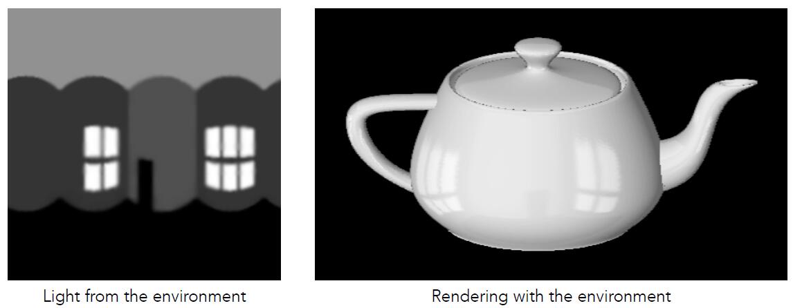
- Environment Map: render with the light from the envrionment as texture
- We suppose the light is static and comes from an infinite distance. We only care about the direction of the light without any depth information.
Info: Classic model in CG: Utah teapot, Stanford bunny, Stanford dragon, Cornell Box
- Spherical Map: Sphere is used to store environment light (map). Unfolding the sphere is texture to render realistic lighting
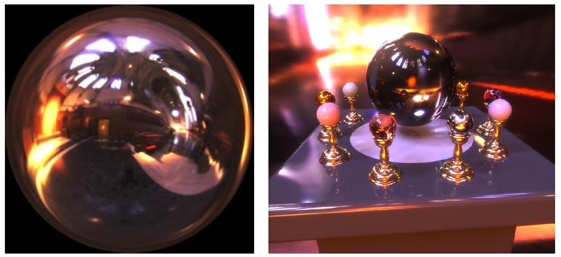
- Sphere texture is prone to distortion at top and bottom parts
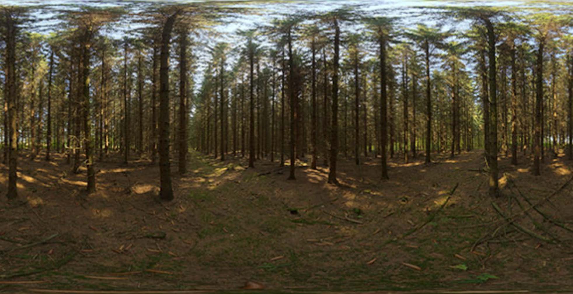
- Sphere texture is prone to distortion at top and bottom parts
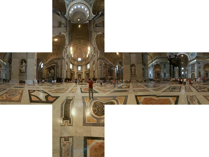
- Cubic Map: A vector map to cube point along the direction. The cube is textured with 6 square texture maps
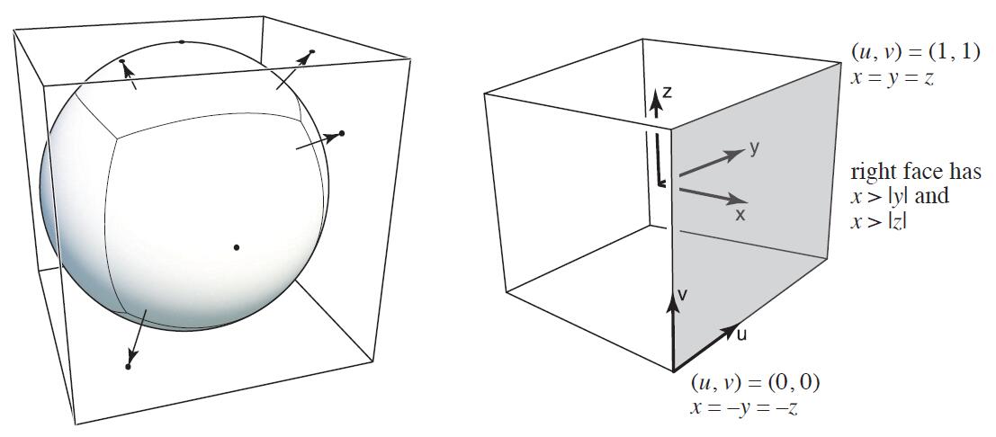
- less distortion
- only need direction to face mapping computation
Bump / Normal mapping
- Previously, textures only represent colors (influence $k_d$ coefficient)
- In fact, textures may store height / normal or other properties
- Fake the detailed geometry, accordingly change the normal and affect shading
- Change how an illuminated surface reacts to light, without modifying the size or shape of the surface
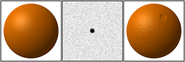
- Add surface detail without adding more triangles
- Preturb surface normal per pixel (for shading computations only)
- “Height shift” per texel defined by a texture
Normal in flatland case
- Flatland (2D): texture in 1D and space in 2D
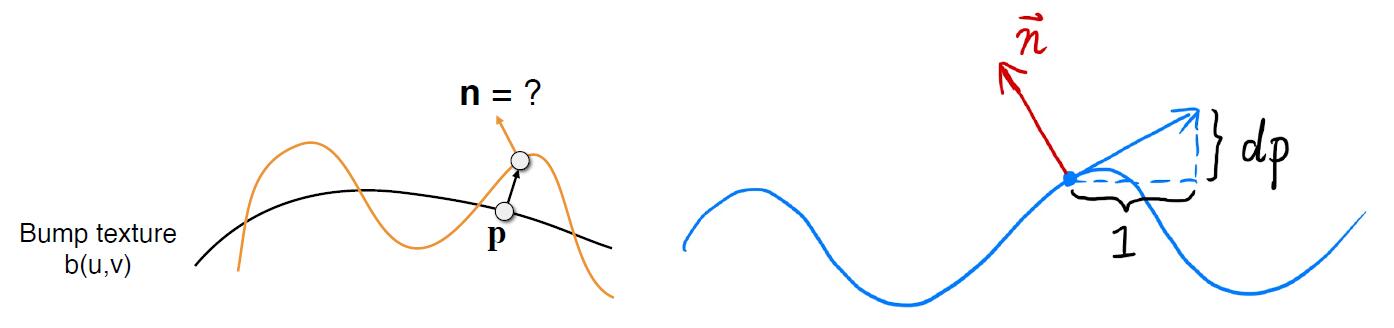
- Suppose original surface normal $\vec p = (0,1)$ directs upward
- Approximate derivative at $p$ is $dp = c * [h(p+1) - h(p)]$
- $c$ is a constant coefficient to scale the influence of bump texture
- Perturbed normal is then $\vec{n_p} = (-dp, 1).normalized()$
- $(1, dp)$ rotate 90 degrees counterclockwise using rotate matrix and normalize
Normal in 3D case
- texture in 2D and space in 3D
- Suppose original surface normal $\vec p = (0, 0, 1)$
-
Approximate derivatives at $p$ are \(dp/du = c_1 * [h(u+1) - h(u)] \\ dp/dv = c_2 * [h(v+1) - h(v)]\)
- Perturbed normal is $\vec{n_p} = (-dp/du, -dp/dv, 1).normalized()$
- // not the cross product result of $(dp/du, 0, 1) \times (dp/dv, 0, 1)$ ?
Note: These are all in local coordinate. Thus, the perturbed normal need to be transformed to world coordinate.
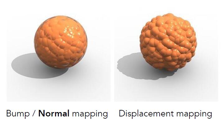
Displacement mapping
- Actually moves the vertices (instead of fake changing the normal only)
- Actual geometric position of vertices over the textured are displaced
- Uses the same texture as in bumping mapping
- Different with Bump / Normal mapping, Displacement mapping permits particular silhouettes, self-occlusion, self-shadowing
- Require primitives in object elaborated and small enough so that the triangles in object catch up with the high frequency in displacement mapping.
- Displacement mapping only changes the vertex properties, thus if the primitive is large and displacement mapping is not able to change the properties inside of the triangle, displacementm mapping will cause poor result.
- In order to render texture with delicated details, the sampling rate must be high enough.
- Subdivision (细分) is needed to introduce more triangles to increase sampling rate.
- Costly computation owing to the large amount of additional geometry
Info: In DirectX on Windows system, dynamic tessellation (动态曲面细分) is self-adaptive techniques to tessellate object geometry in displacement mapping stage, which dynamically splits the primitives of object into smaller part of triangle to match the frequency requirements of displacement mapping.
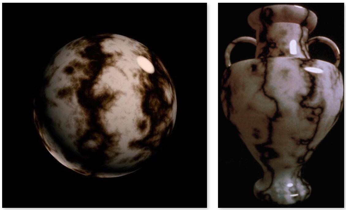
Noise function Texture
- 3D procedural noise and solid modeling produce texture.
- Defining the noise function in 3D space, each point of the texture spreading over this space can be calculated by analysis formula of the noise and corresponding operations (binaryzation, linear operation).
Perlin noiseis a good example of noise function to generate marble crack, mountain fluctuation etc.
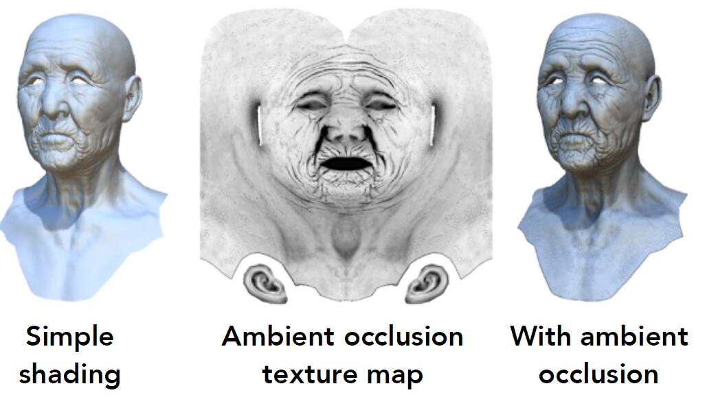
Precomputed Shading
- Texture provide precomputed shading
- Precomputed ambnient occlusion and shadow provided by the texture to save time of calculating shadow and occlusion later
3D Texture and Volumn Rendering
- Texture can be generalized to 3D space, storing the information and properties (far more than colors) which is to be used and processed in Shader program.