Geometry, Implicit & Explicit Geometry, Curve, Surface, Subdivision, Mesh Simplification
Geometry
- Implicit Geometry
- algebraic surface
- level sets
- distance functions
- …
- Explicit Geometry
- point cloud
- polygon mesh
- subdivision, NURBS
- …
- Each choice best suited to a different task/type of geometry
Implicit Representations of Geometry
- Based on classifying points: Points satisfy some specified relationship, without given coordinate
- E.g. sphere: all points in 3D, where $x^2+y^2+z^2=1$
- More generally, $f(x, y, z) = 0$
Take $f(x, y, z)=\left(2-\sqrt{x^{2}+y^{2}}\right)^{2}+z^{2}-1$ as an example:
- Implicit Surface sampling can be hard
- What points lie on $f(x, y, z) = 0$
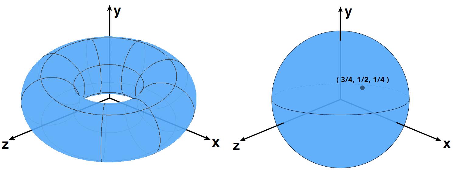
Take $f(x, y, z)=x^{2}+y^{2}+z^{2}-1$ as an example:
- Implicit Surface inside/outside test is easy
- Is $(3/4, 1/2, 1/4)$ inside the sphere?
- Just plug it in $f(x, y, z) = -1/8 < 0$, so Inside
Implicit Geometry
- Implicit Algebraic Surfaces
- Constructive solid geometry
- Level set methods
- Fractals
Algebraic Surfaces
- Surface is zero set of a polynomial in x, y, z
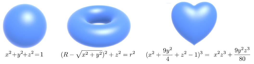
- But how about using polynomial to represent a more complext object as a cow?
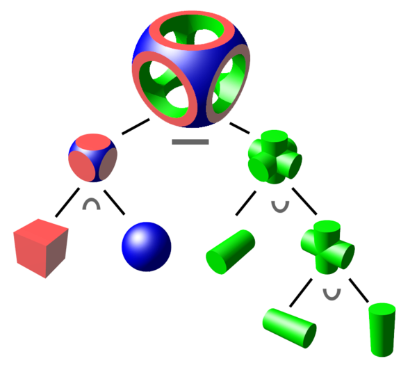
Constructive Solid Geometry
- Constructive Solid Geometry (CSG): Combine implicit geometry via Boolean operations
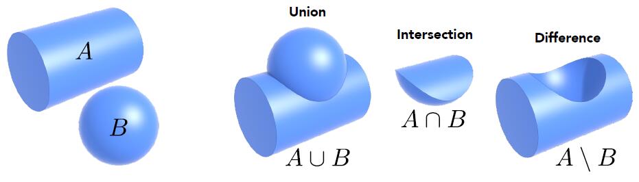
- Use CSG and operation to define complex geometry
Distance Functions
-
Signed Distance Functions (SDF): determines the distance of a given point $x$ from the boundary of $\omega$. The function has positive values at points $x$ outside $\omega$, it decreases in value as $x$ approches the boundary of $\omega$ where the signed distance function is zero.
-
Instead of Booleans, gradually blend surfaces together using Distance functions:
- Give minimum distance (could be signed distance) from anywhere to object
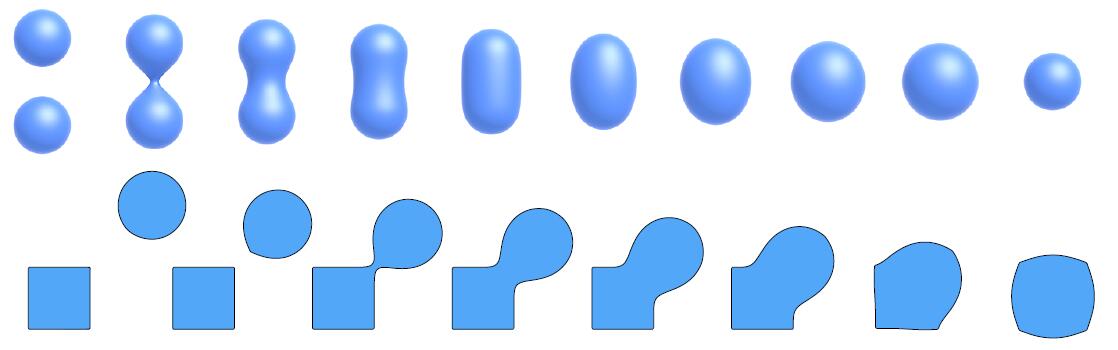
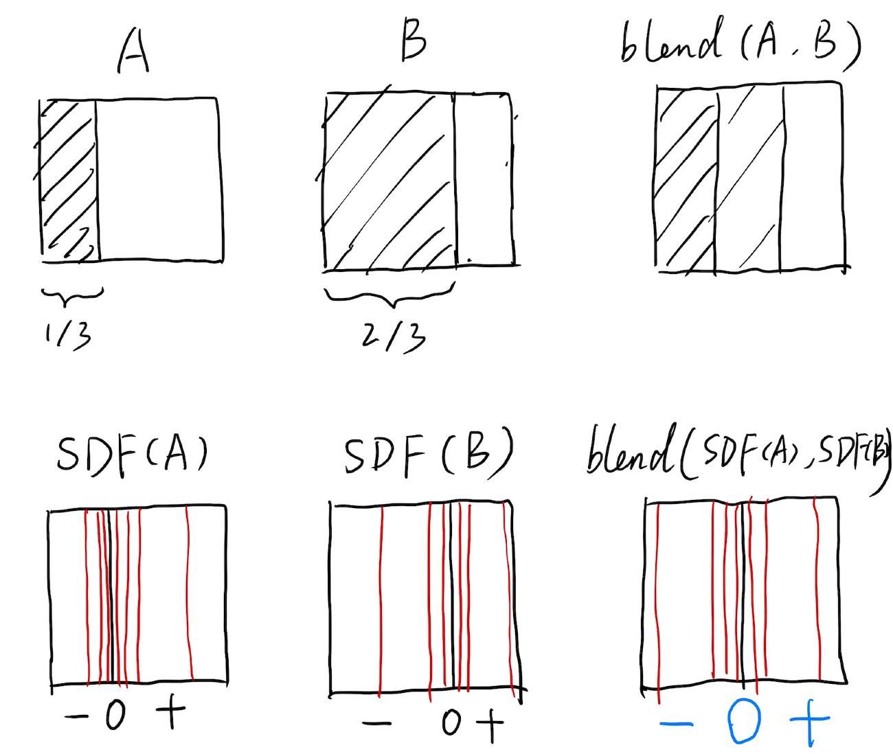
- An Example: Blending (linear interp.) a moving boundary
- The above row describes the normal blending of A and B region, which results A overlaps B
- The below row describes the blending using SDF, similar to superposition of the electric field of two same point charges, which results the zero plane right in the middle of A and B
-
Blending any two distance functions: every point in the space can be represented as distance function, blending of two objects in the space is to sum up two distance functions. The boundary forms when the distance function is 0
-
More details about distance function, SDF code about various primitives and useful tutorial
Level Set Methods
- For Distance Function method, closed-form equations (解析式) are sometimes hard to describe complex shapes.
- Level Set Methods performs numerical computations involving curves and surfaces on a fixed Cardesian grid without having to parameterize objects.
- Level Set Methods is to store a grid of values approximating function.
- The central idea is same to SDF: find the boundary where the value is 0.
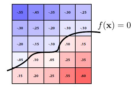
- Surface is found where interpolated values equal zero
-
Provides much more explicit control over shape (like a texture)
- Level set encodes distance to air-liquid boundary to simulate physical scene of water dropping, constant tissue density to image medical data like CT, MRI etc.
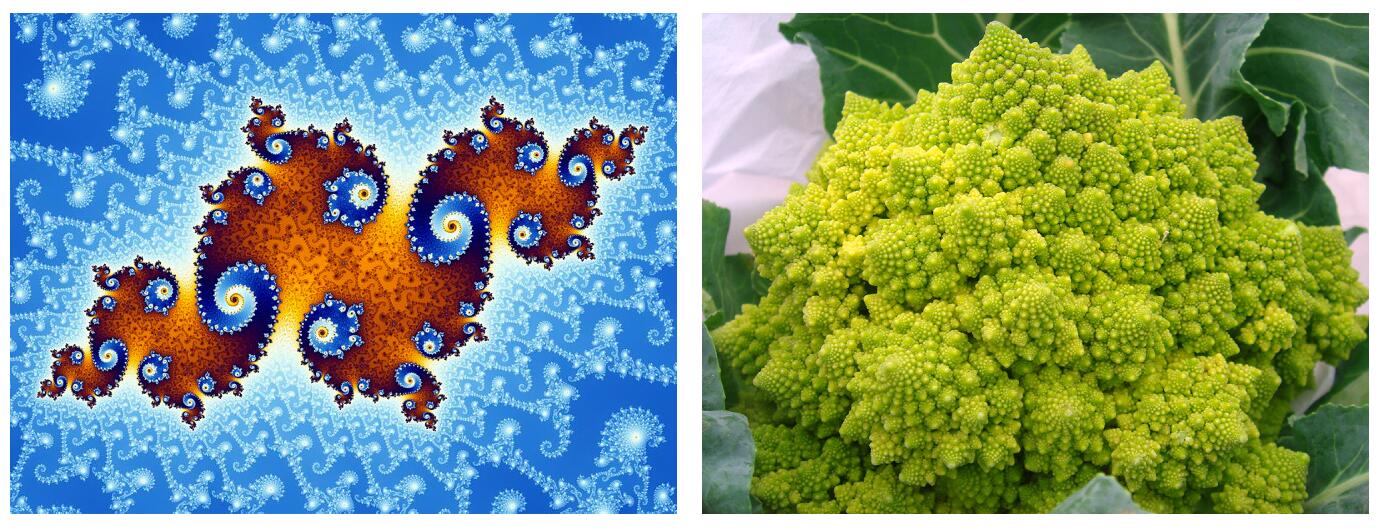
Fractal
- Self-similarity, detail at all scales
- Hard to control shape
- Sometimes cause the drastic aliasing due to the high frequency of variation
Pros & Cons
- Pros
- compact description (a function), benefit for storing
- queries easy (inside object, distance to surface)
- good for ray-to-surface intersection
- easy to handle changes in topology (e.g. fluid)
- Cons
- difficult to model complex shapes
Explicit Representations of Geometry
- All points are given directly or via parameter mapping
- Given any $(u,v)$ coordinate, $(x, y, z)$ can be mapped
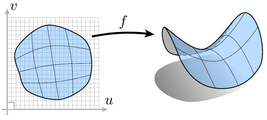
Take $f(u, v)=((2+\cos u) \cos v,(2+\cos u) \sin v, \sin u)$ as an example
- Explicit Surface sampling is easy
- What points lie on this surface: Just plug in $(u,v)$ values
- Take $f(u, v)=(\cos u \sin v, \sin u \sin v, \cos v)$ as an example
- Is $(3/4, 1/2, 1/4)$ inside the sphere?
- No Best Representation: depends on tasks
Explicit Geometry
- triangle meshes
- Bezier surfaces
- subdivision surfaces
- NURBS
- point clouds
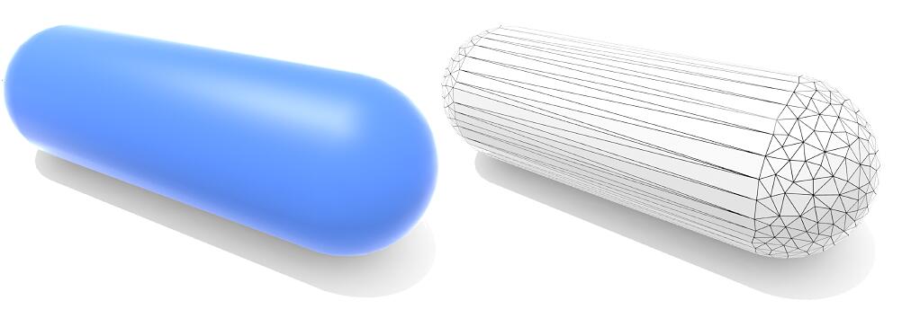
Polygon Mesh
- Store vertices & polygons (often triangles or quads)
- Easier to do processing / simulation, adaptive sampling
- More complicated data structures
- Perhaps most common representation in graphics
- The Wavefront Object File (.obj) Format
- a text file that specifies vertices, normals, texture coordinates and their connectivities
Point Cloud
- Easiest representation: list of points $(x, y, z)$
- Easily represent any kind of geometry
- Useful for large datasets (>> 1 point/pixel)
- Often converted into polygon mesh
- Difficult to draw in undersampled (采样不足的) regions
Curves
Bézier Curve
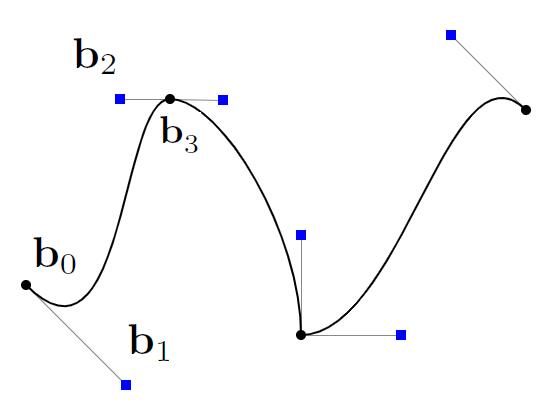
- Defining Cubic Bézier Curve With Tangent
- Start point and the end point is $b_0$ and $b_2$
- Tangent of start and end is the tangent at $b_0$ and $b_2$
Note: Bézier Curve is a representation of explicit geometry since it is way of parameter mapping
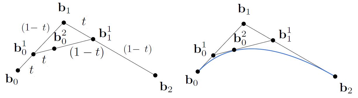
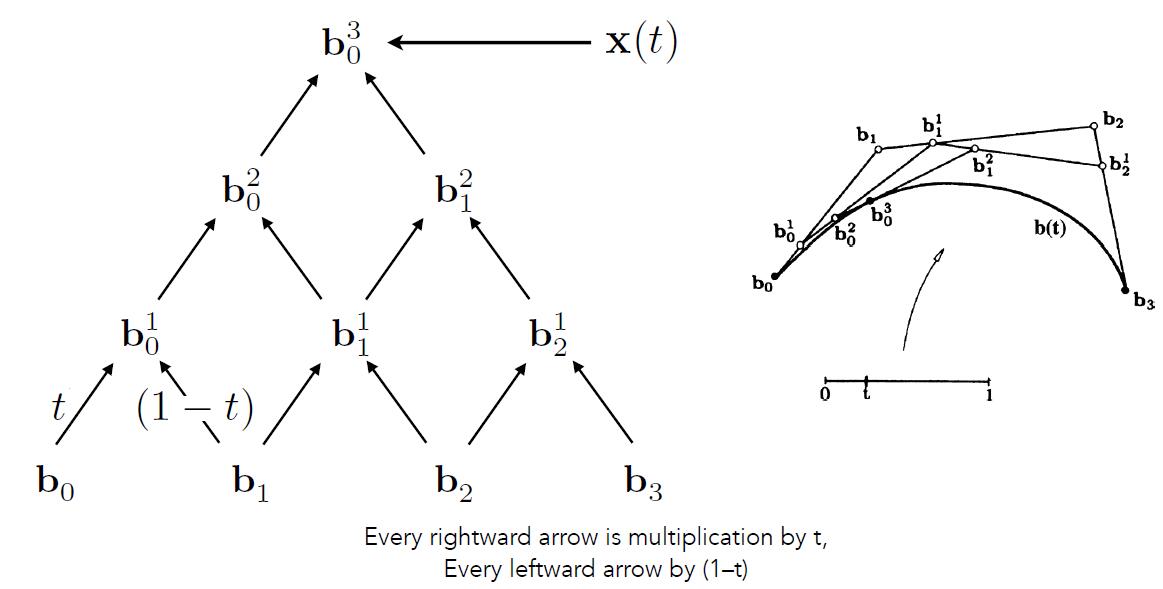
de Casteljau Algorithm
- Evaluate Bézier Curve
- Consider three points (quadratic Bezier)
- Insert a point using linear interpolation
- Insert on both edges
- Repeat recursively until only one intermediate point exists
- Run the same algorithm for every $t$ in $[0, 1]$
Algebraic Formula
- de Casteljau Algorithm gives a pyramid of coefficients
- General Algebraic Formula
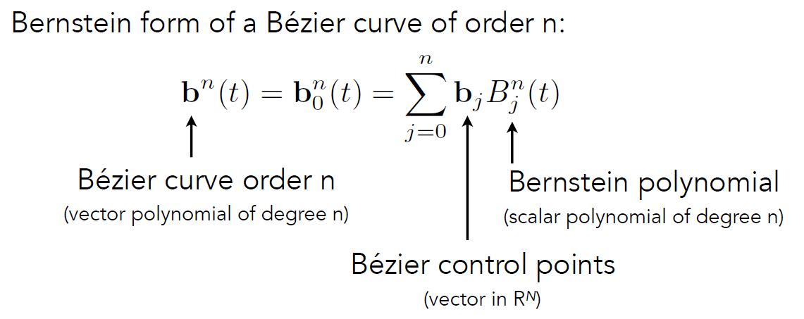
- Bernstein polynomials
- For each $t$ moment, the sum of Bernstein Polynomials is 1. Drawing a vertical line at any $t$ moment, the sum of the y-coordinate of the intersection with the curve is 1.
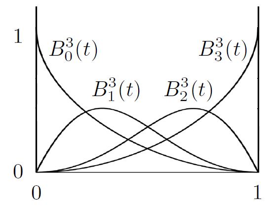
- assume $n=3$ in $R^3$:
- The tangent of the curve in cubic case: the slope for Bézier Curve is the derivative with respect to $t$
Properties of Bézier Curve
- Interpolate endpoints: Start from $B_0$, end at $B_n$
- Tangent to end segment: In cubic case $\mathbf{b}^{\prime}(0)=3\left(\mathbf{b}_{1}-\mathbf{b}_{0}\right)$, $\mathbf{b}^{\prime}(1)=3\left(\mathbf{b}_{3}-\mathbf{b}_{2}\right)$
- Transform curve by transforming control points
- Since the Bézier Curve is the result of linear combinations
- But it doesn’t work for projection transformation
- Convex hull (凸包) property
- Curve is within convex hull of control points
- Convex hull is a concept in computational geometry. Briefly, it can be thought of as a rubber band that fits around all the points in 2D space
Piecewise Bézier Curve
- Higher-order (high-degree 高阶) Bézier Curve is hard to control: Instead, Piecewise (逐段的) Bézier Curve is put forward
- Chain many low-order Bézier Curves
- Piecewise cubic Bézier Curve is the most common technique and widely used in Apps (Illustrator, SVG, etc.)
- For Cubic Curve, each four pair of point defining a piece of Bézier Curve
- The curve is continuous when each piece of curve is connected
- The curve is smooth when the connection of each curve is smooth
- Smooth: the derivative (slope) of the previous ending point of the curve is the same as the subsequent curve.
Samemeans both direction and the amount of value.
- Smooth: the derivative (slope) of the previous ending point of the curve is the same as the subsequent curve.
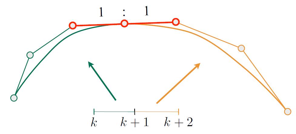
- Continuity
- $C^0$ continuity: $a_n = b_0$
- $C^1$ continuity: $a_n = b_0 = \frac{1}{2}(a_{n-1}+b_1)$
Spline
- Spline (样条): a continuous curve constructed so as to pass through a given set of points and have a certain number of continuous derivatives
- In short, a curve under control directly
B-splines
- B-spline: Short for basis splines
- Require more information than Bézier Curve curbes
- Satisfy all important properties that Bézier Curve have (i.e. superset)
- # TODO: refer to Shi-Min Hu’s course
NURBS
- # TODO: refer to Shi-Min Hu’s course
Surface
Bézier Surface
- Extend Bézier curves to surfaces under control of 2D control points
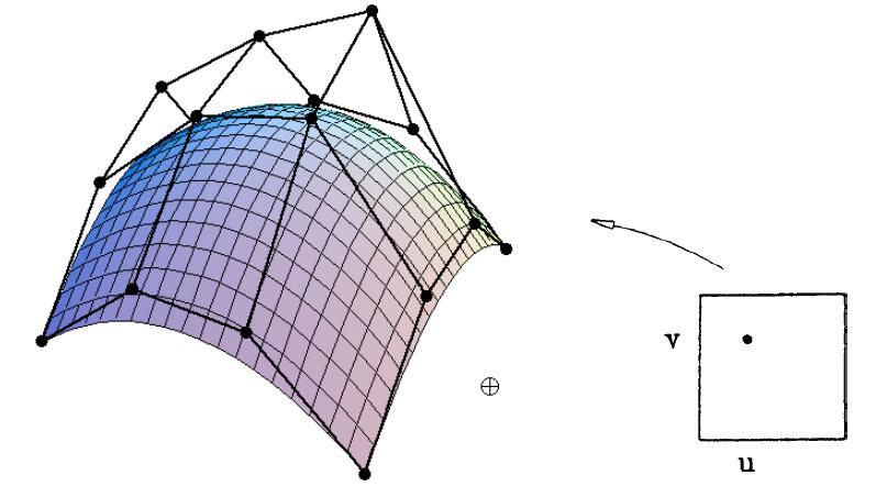
- For Bicubic Bézier surface patch, evaluate surface position for parameters $(u, v)$
- $(u, v)$ is parameters to describe two-dimensional $t$, which proves again that Bézier (parameter mapping) is explicit geometry representation
- Input: 4x4 control points
- Output: 2D surface parameterized by $(u, v)$ in $[0,1]^2$
- Bicubic operation: similar to ‘Bicubic interpolation’
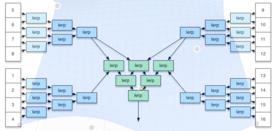
- Separable 1D de Casteljau Algorithm
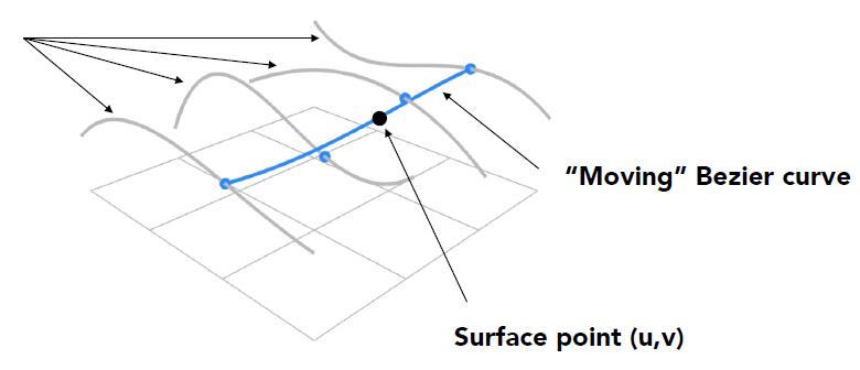
- Goal: evaluate surface position corresponding to $(u, v)$
- (u, v)-separable application of de Casteljau algorithm
- Use de Casteljau to evaluate point $u$ on each of the 4 Bézier curves in $u$. This gives 4 control points for the ‘moving’ Bézier curve
- Use 1D de Casteljau to evaluate point $v$ on the ‘moving’ curve
TIP: piecewise (片段) in 2D curve vs patch (片) in 3D surface
- #TODO: Continuity
Mesh Operations
- Mesh (网格) Operations: Geometry Processing
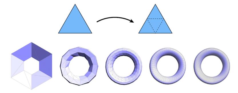
- Mesh subdivion (细分): increase resolution (upsampling)
- Mesh simplification: decrease resolution (downsampling) while preserving shape/appearance
- Mesh regularization: modify sample distribution to improve quality
Subdivision
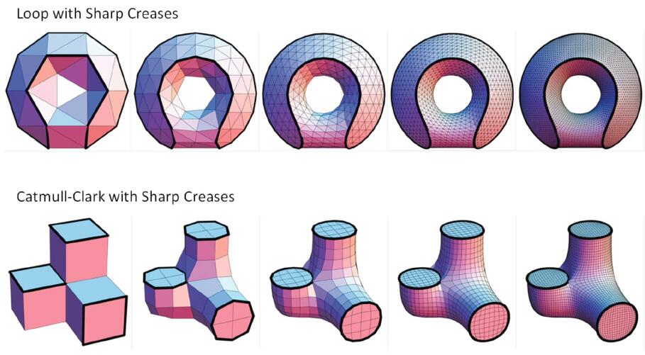
Loop Subdivision
- Common subdivison rule for triangle meshes
- First create more triangles (vertices)
- Second, tune their positions
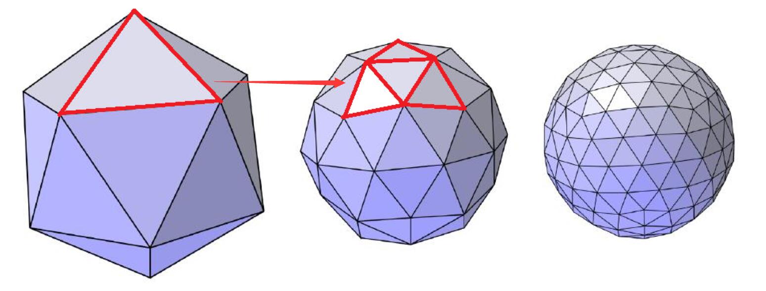
- Split each triangle into four
- Assign new vertex positions according to weights
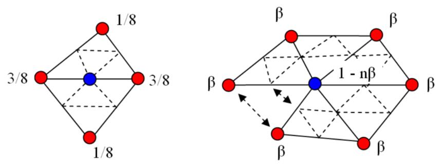
- New / old vertices updated differently
- For new vertices: $ v = 3/8 * (A+B) + 1/8 * (C+D)$
- For old vertices: \(\begin{aligned}v=(1-\beta) * original\_position + \beta * \sum^{n} neighbour\_position, \end{aligned} \\ where:\quad \beta=\left\{\begin{array}{l}\frac{3}{8 \mathrm{n}},\quad when\quad n>3 \\ \frac{3}{16},\quad when\quad \mathrm{n}=3\end{array}\right.\)
Tip: $n$ is vertex degree. In graph theory, the degree of a vertex is the number of edges that are incident to the vertex.
Note: Loop is family name of the founder Charles Loop of Loop Subdivision, so it has nothing to do with looping.
Catmul-Clark Subdivision
- Catmul-Clark subdivision is more general than Loop Subdivision since Catmul-Clark Subdivision can handle mesh with not only triangles but quadrangles.
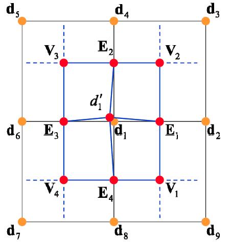
- Each subdivision step:
- Keep all original vertex $d$
- Add vertex in each face $V_i$
- Add midpoint on each edge $E_i$
- Connect all new vertices
- After each subdivision
- No extraordinatry (奇异点) vertices (degree != 4) left
- No non-quad face left
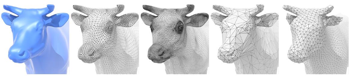
Mesh Simplification
- Goal: reduce number of mesh elements while maintaining the overall shape
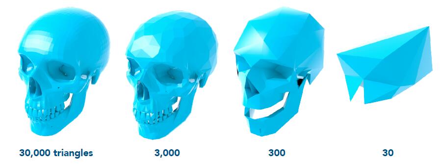
- Difficulty: For image simplification (downsampling), take Mipmap as an example, which can be performed by reducing the image resolution for several times, image pyramid (mip hierarchy) is used to represent different level of vision field. While for the geometry, it is difficult to use the similar pattern to divide the hierarchy of geometry, like how to make the number of geometric mesh change smoothly from far to near.
Edge Collapsing
- Suppose we simplify a mesh using edge collapsing
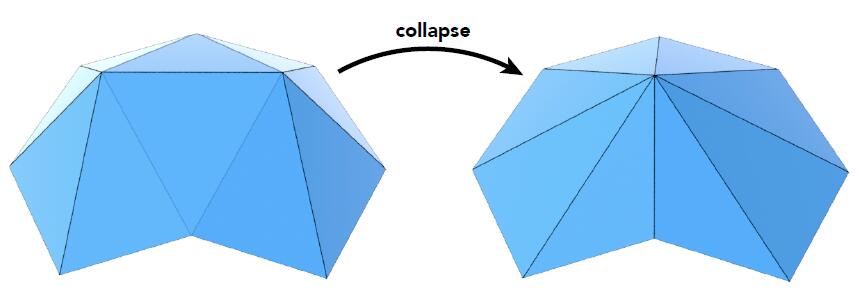
- Geometric error will be introduced by simplification .
- Comparing to average and median simplification, error of quadric is minimum.
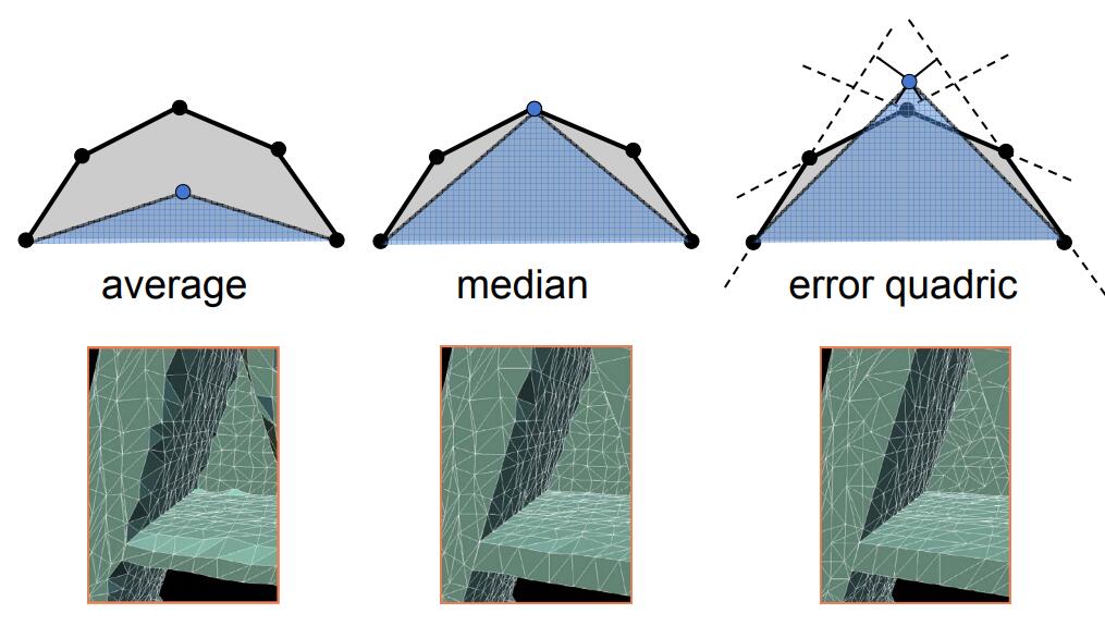
- Quadric Error Metrics (二次误差度量)
- Not a good idea to perform local averaging or median of vertices
- Quadric error: new vertex should minimize its sum of square distance (L2 distance) to previously related triangle planes
- Idea: choose point that minimizes quadric error
- Suppose squared distance of point $p$ to plane $q$
Note: $q$ is a regularized parameter of plane, where $a^2+b^2+c^2 = 1$.
- Sum distances to planes $q_i$ of vertex’ neighbouring triangles
- Point $p^{\star}$ that minimizes the error satisfies
- Which turn into the optimization problem
- Simplification via Quadric Error: assign score with quadric error metric (Garland & Heckbert 1997)
- Approximate distance to surface as sum of distances to planes containing triangles
- Assign score with quadric error metric for each edge of the total geometric figure
- Sort the score of each edge
- Select the smallest score with least quadric error metric and perform edge collapsing
- Update the corresponding changed edges with new quadric error
- Iteratively execute until the simplification reaches condition
Note: For each step, the edge corresponding to the least quadric error is selected to be collasped. Clearly, this is a way of reaching local optimum for each step to achieve global optimum, namely greedy strategy. However strictly speaking, this approch does not prove that the global optimal solution can be reached, but this insignificant error is allowed by default in CG.