The Notes of Computer Graphics Ⅸ

Advanced Ray Tracing, Radiometry, BRDF, Path Tracing

Radiometry

• Motivation: Blinn-Phong is experienced model and light intensity corresponding to the amount of shading is not explained well, the output is not realistic but plastic. Whitted-style ray tracing sometimes doesn’t give correct result, especially involving how much light energy is refracted and reflected, and how much the rest is absorbed by the material, etc.
  • All the answers can be found in radiometry!
• Measurement system and units for illumination
• Accurately measure the spatial properties of light (not temperal dimension, we still suppose light travel in straight line with out wave property)
  • New terms: Radiant flux, intensity, irradiance, radiance (辐射通量, 光强, 照度, 亮度)
• Perform lighting calculations in a physically correct manner

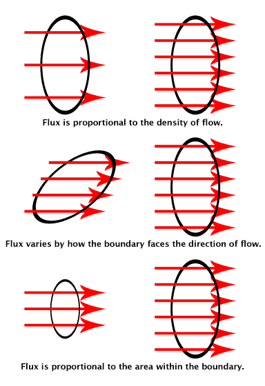
Radiant Energy and Flux

• Radiant energy: the energy of electromagnetic radiation. It is measured in units of joules, and denoted by the symbol:

• Radiant flux (radiant power, luminous flux): the energy emitted, reflected, transmitted or received, per unit time.
  • Flux: photons flowing through a sensor in unit time

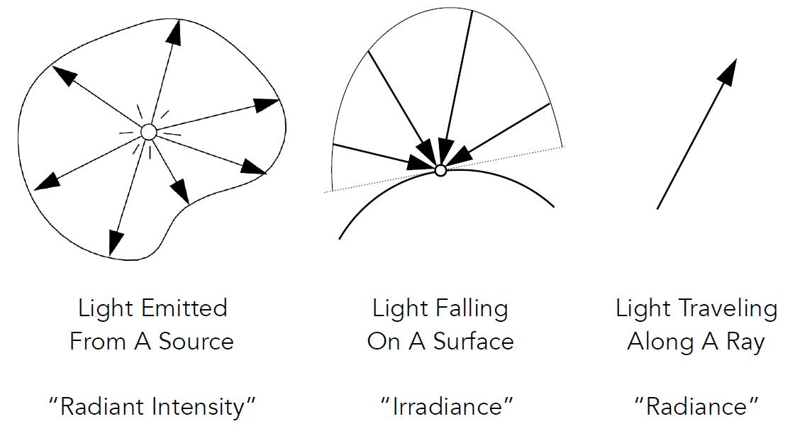
Radiant Intensity

• Radiant Intensity: The radiant (luminous) intensity is the power per unit solid angle emitted by a point light source.

• The candela is one of the seven SI base units

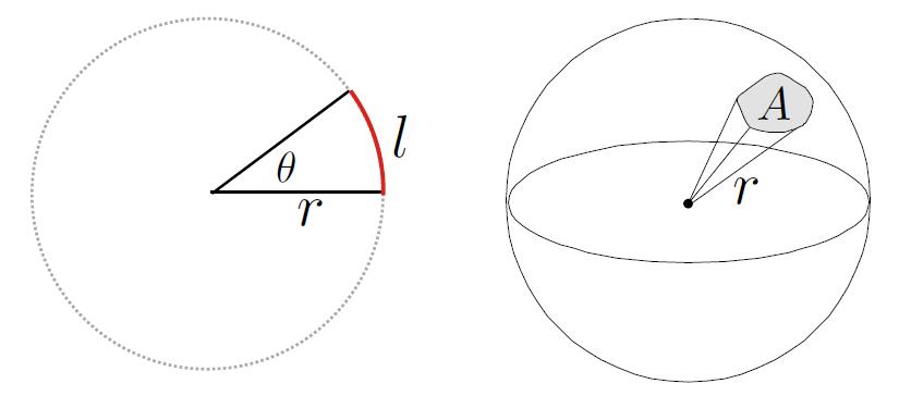
Angles and Solid Angles

• Angle: ratio of subtended arc length on circle to radius
  • $\theta = l / r$
  • Circle has $2\pi$ radians
• Solid angle: ratio of subtended area on sphere to radius squared
  • $\omega = A / r^2$
  • Sphere has $4\pi$ steradians

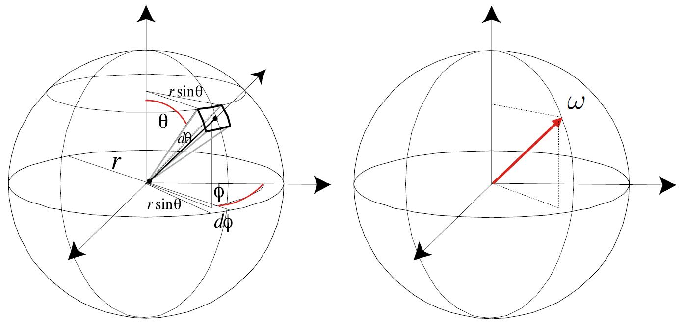
• Differential Solid Angles
  • Direction vector $\omega$ to denote direction vector of unit length
  • $\theta$ : elevation, zenith angle (仰角)
  • $\phi$ : azimuth, azimuth angle (方位角)
  \[\mathrm{d} A =(r \mathrm{~d} \theta)(r \sin \theta \mathrm{d} \phi) =r^{2} \sin \theta \mathrm{d} \theta \mathrm{d} \phi\] \[\mathrm{d} \omega =\frac{\mathrm{d} A}{r^{2}}=\sin \theta \mathrm{d} \theta \mathrm{d} \phi\]
  • Sphere: $S^{2}$

• Isotropic Point Source

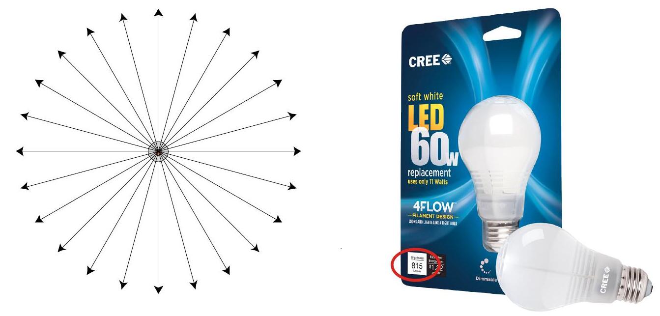
• Modern LED Light
  • Output: 815 lumens (11W LED replacement paifor 60W incandescent)
  • Radiant intensity (assume isotropic) = 815 lumens / 4π sr = 65 candelas

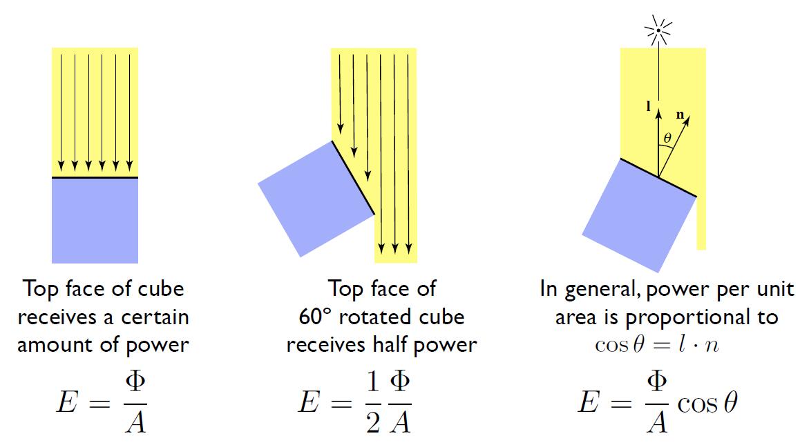
Irradiance

• Irradiance: the power per (perpendicular / projected) unit area incident on a surface point.

• The lux is SI derived unit of illuminance, measuring luminous flux per unit area.

• Irradiance at surface is proportional to cosine of angle between light direction and surface normal
  • Recall Lambert’s Cosine Law

Tip: Analogous Irradiance to Electric field intensity, Radiant flux to Magnetic Flux.

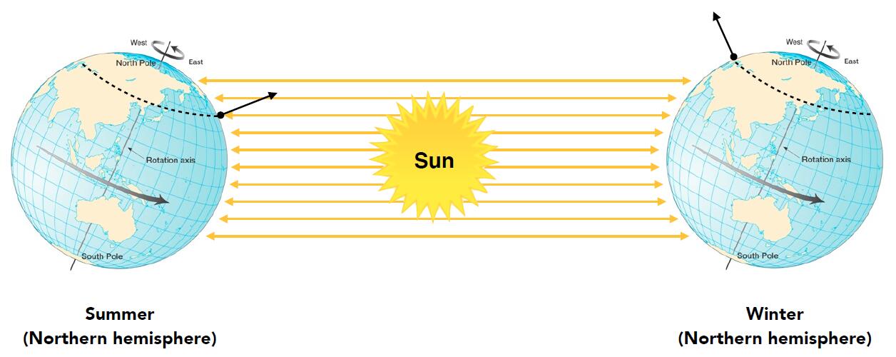
• The reason why we feel cold and hot in different seasons
  • Earth’s axis of rotation: ~23.5° off axis
  • Give rise to the different Solar elevation angle

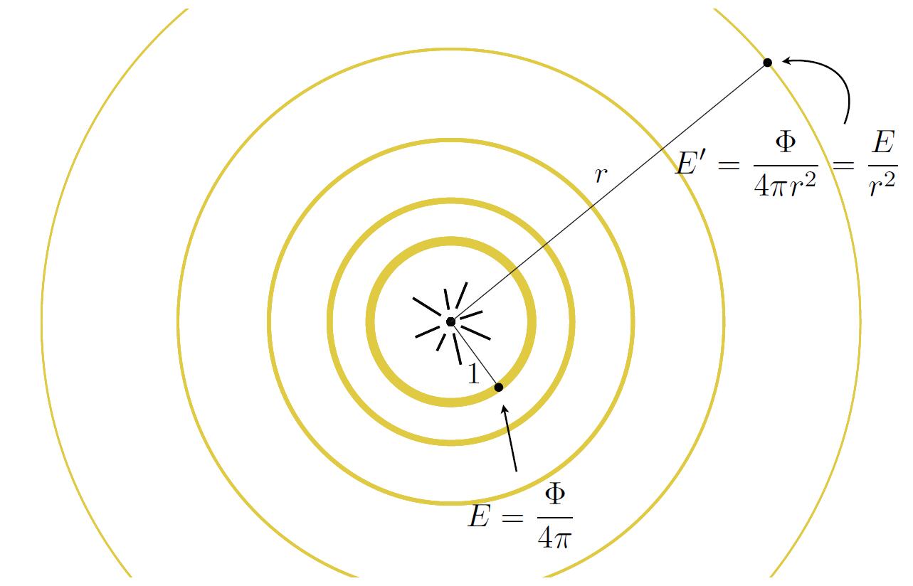
• Correction of Irradiance Falloff
  • Assume light is emitting power $\Phi$ in a uniform angular distribution
  • Compare irradiance at surface of two spheres

Radiance

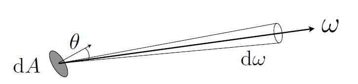
• Radiance (luminance): the power emitted, reflected, transmitted or received by a surface, per unit solid angle, per projected unit area.
  • Radiance is the fundamental field quantity that describes the distribution of light in an environment
  • Radiance is the quantity associated with a ray
  • Rendering is all about computing radiance

• $\cos\theta$ accounts for projected surface area
• The nit, the candela per square metre, is the derived SI unit of luminance.

• Recall
  • Irradiance: power per projected unit area
  • Intensity: power per solid angle
  • Radiance: power per solid angle, per projected unit area
• Thus
  • Radiance: Irradiance per solid angle
  • Radiance: Intensity per projected unit area

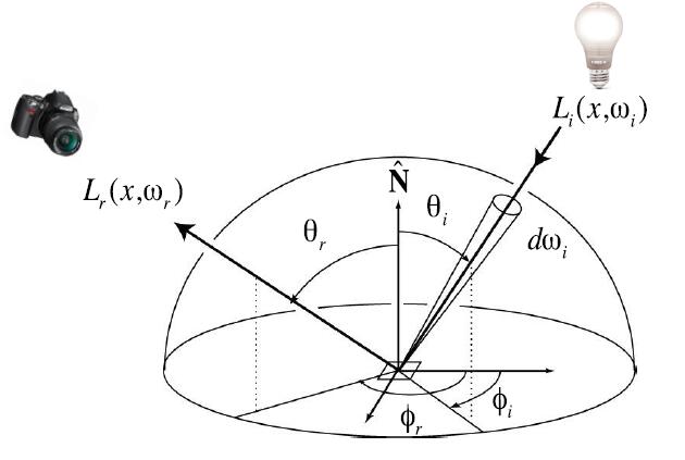
Incident Radiance

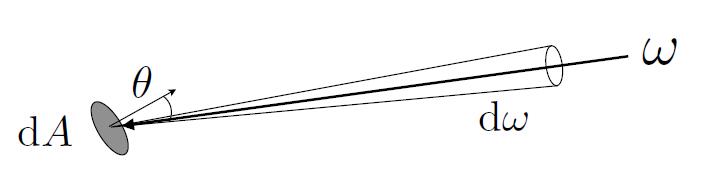
• Incident Radiance: the irradiance per unit solid angle arriving at the surface
  • It is the light arriving at the surface along a given ray (point on surface and incident direction).

Exiting Radiance

• Exiting Radiance: the intensity per unit projected area leaving the surface
  • For an area light, it is the light emitted along a given ray (point on surface and exit direction).

Irradiance vs. Radiance

• Irradiance: total power received by area $dA$
• Radiance: power received by area $dA$ from direction $d\omega$

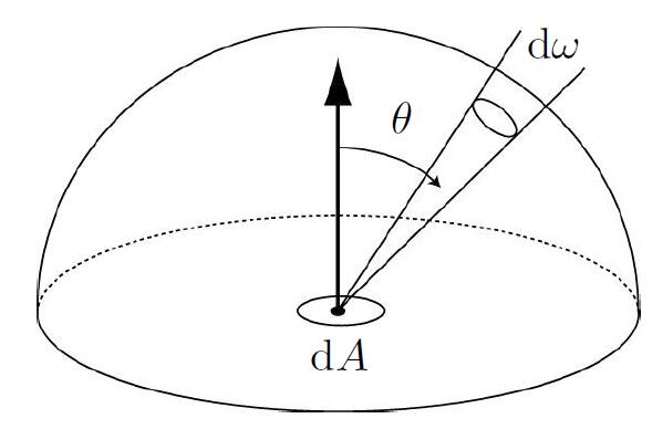
• Unit Hemisphere $H^2$

Bidirectional Reflectance Distribution Function

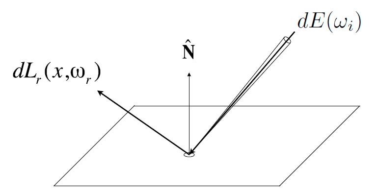
• Radiance from direction $\omega_i$ turns into the power $E$ that $dA$ receives
• The npower $E$ will become the radiance to any other direction $\omega_o$

• Differential irradiance incoming: $d E\left(\omega_{i}\right)=L\left(\omega_{i}\right) \cos \theta_{i} d \omega_{i}$

• Differential radiance exiting (due to $dE(\omega_i)$): $dL_r(\omega_r)$

• BRDF can be understanded in the way of energy distribution after the point on the surface absorbs the energy from directions all around and then reflects.

  • For the specular reflection, BRDF specifies the reflected energy is mostly on the reflection direction
  • For the diffuse reflection, BRDF specifies the reflected energy will distributed amoung all directions around.

BRDF

• Bidirectional Reflectance Distribution Function (BRDF): represents how much light is reflected into each outgoing direction $\omega_r$ from each incoming direction

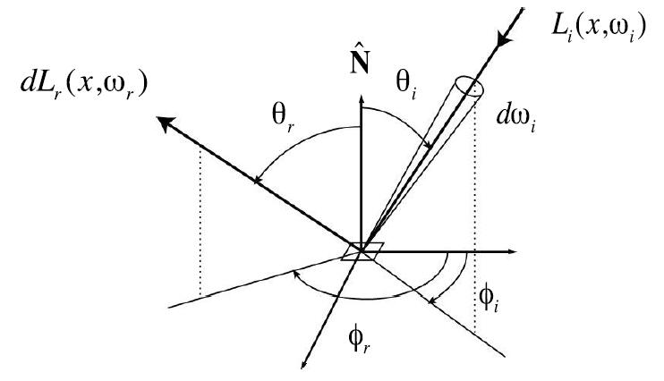
• Conclusion: The BRDF, the ratio of exitant radiance to incident irradiance, is to characterize the directional properties of how a surface reflects light, which is independent of the strength of the light.
  • In fact, we use cosine irradiance collector to measure incident irradiance, conical baffler to measure received radiance, and calculate the BRDF corresponding to the surface/texture by dividing the two. More info, and later notes
  • In a word, BRDF describes how the light interacts with the object. Accordingly, BRDF describes the property of the texture.
• The quantity is between zero and one for reasons of energy conservation.

Reflection Equation

• Consider BRDF only takes one direction of incident light, thus integral light (energy) from all directions of hemisphere will get the entire light source directing to the reflection point.
  • Understand in discrete way: traverse solid angles on the hemisphere, each incident solid angle will make contribution to the radiance of one specified direction. Sum these up will get the entire contribution, that is received energy.

• Challenege: recursion
  • Reflected radiance $L_{r}\left(\mathrm{p}, \omega_{r}\right)$ on the left hand depends on incoming radiance $L_{i}\left(\mathrm{p}, \omega_{i}\right)$ on the right hand.
  • But incoming radiance depends on reflected radiance at another point in the scene.
    • Incoming radiance is not limited to the light source, but reflected light etc.

Rendering Equation

• Rewrite the reflection equation by adding an Emission term $L_{e}\left(p, \omega_{o}\right)$ to make it general:

Caveat: we assume that all directions are pointing outwards, and field of integration is hemisphere, which is the reason for $\cos\theta$ replacing $max(\cos\theta, 0)$.

• Volume rendering equation is a more general form of rendering equation.

• The solution of renderings equation will be narrated in the following part.

• Understanding of the rendering equation

  • for the single light source
  \[\underset{\\ \quad \\ Reflected\ Light \\ (Output\ image)}{L_{r}\left(x, \omega_{r}\right)}= \underset{\\ \quad \\ Emission}{L_{e}\left(x, \omega_{r}\right)} + \underset{\\ \quad \\ Incident \ Light \\ (from\ light \\ source)}{L_{i}\left(x, \omega_{i}\right)} \underset{\\ \quad \\ BRDF}{f\left(x, \omega_{i}, \omega_{r}\right)} \underset{\\ \quad \\ Cosine\ of \\ Incident\ angle}{\left(\omega_{i}, n\right)}\]
  • for the multiple light sources
  \[\underset{\\ \quad \\ Reflected\ Light \\ (Output\ image)}{L_{r}\left(x, \omega_{r}\right)} = \underset{\\ \quad \\ Emission}{L_{e}\left(x, \omega_{r}\right)} + \sum \underset{\\ \quad \\ Incident \ Light \\ (from\ light \\ source)}{L_{i}\left(x, \omega_{i}\right)} \underset{\\ \quad \\ BRDF}{f\left(x, \omega_{i}, \omega_{r}\right)} \underset{\\ \quad \\ Cosine\ of \\ Incident\ angle}{\left(\omega_{i}, n\right)}\]
  • for the planar light sources
  \[\underset{\\ \quad \\ Reflected\ Light \\ (Output\ image)}{L_{r}\left(x, \omega_{r}\right)} = \underset{\\ \quad \\ Emission}{L_{e}\left(x, \omega_{r}\right)} + \int_\omega \underset{\\ \quad \\ Incident \ Light \\ (from\ light \\ source)}{L_{i}\left(x, \omega_{i}\right)} \underset{\\ \quad \\ BRDF}{f\left(x, \omega_{i}, \omega_{r}\right)} \underset{\\ \quad \\ Cosine\ of \\ Incident\ angle}{\cos \theta_i d\omega_i}\]
  • for the surfaces with reflected light (interreflection)
  \[\underset{\\ \quad \\ Reflected\ Light \\ (Output\ image) \\ \quad \color{red}{Unkown}}{L_{r}\left(x, \omega_{r}\right)} = \underset{\\ \quad \\ Emission \\ \color{blue}{Known}}{L_{e}\left(x, \omega_{r}\right)} + \int_\omega \underset{\\ \quad \\ Reflected\ light \\ from\ others \\ \quad \color{red}{Unkown}}{L_{r}\left(x^\prime, -\omega_i\right)} \underset{\\ \quad \\ BRDF \\ \color{blue}{Known}}{f\left(x, \omega_{i}, \omega_{r}\right)} \underset{\\ \quad \\ Cosine\ of \\ Incident\ angle \\ \color{blue}{Known}}{\cos \theta_i d\omega_i}\]

  Tip: $-\omega$ is because the light direction is pointing opposite of the incident direction with regards to $x^\prime$.

  • which is the canonical form of Fredholm Integral Equation of second kind
  \[\underset{\\ \quad \\ Radiance \\ \color{red}{Unkown}}{\color{red}{I(u)}} = \underset{\\ \quad \\ Emission}{e(u)} + \int \underset{\\ \quad \\ Radiance\\ from\ others \\ \color{red}{Unkown}}{\color{red}{I(v)}} \underset{\\ \quad \\ \quad Kernel\ of\ equation \\ \quad Light\ Transport\ Operator}{\boxed{K(u, v)dv}}\]

  Tip: Use substitution rule for integrals from the current object to the object of reflected light source will achieve $d\omega_i$ to $dv$, which will be detailed in solution part.

  • which can be discretized to a simple matrix equation or system of simultaneous linear equations, where $L,\ E$ are vectors, $K$ is the light transport matrix (reflection operator)
  \[\color{red}{L} = E + K\color{red}{L}\]
  • rearrange terms and use taylor expassion
  \[\begin{aligned}\color{red}{L}&=E+K\color{red}{L} \\ I\color{red}{L}-K\color{red}{L} &= E \\ (I-K)\color{red}{L} &= E \\ \color{red}{L} &= (I-K)^{-1}E \\ \color{red}{L} &= (I + K + K^2 + K^3 + ...)E \\ \color{red}{L} &= E + KE + K^2E + K^3E + ...\end{aligned}\]
  • final form of ray tracing is
  \[L = \color{orange}{E + KE} + K^2E + K^3E + ...\]
  • understanding of the expression
    • $K$ : Reflection operator
    • $E$ : Emission directly from light sources
    • $KE$ : Direct illumination on surfaces
    • $K^2E$ : Indirect illumination (One bounce indirect, mirros, refraction)
    • $K^3E$ : Two bounce indirect illumination
    • $\color{orange}{E + KE}$: Direct illumination is all the shading in rasterization can do
  • Global illumination: the union of all direct and indirect light

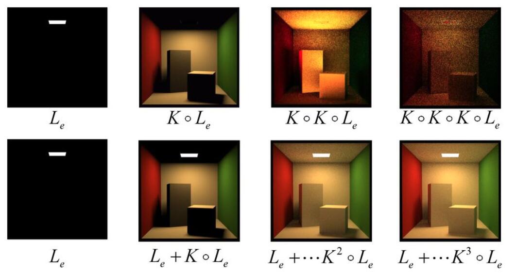
• The more bounce of illumination, the more realistic. When the bounce of illumination goes to infinity, the image finally becomes factual as in the real world.

Mathematics Foundation

Fredholm Integral Equation

• Equation of the first kind

  \[g(t)=\int_{a}^{b} K(t, s) f(s) \mathrm{d} s\]
  • Given the continuous kernel function $K$ and the function $g$, to find the function $f$

• Equation of the second kind

  \[\varphi(t)=f(t)+\lambda \int_{a}^{b} K(t, s) \varphi(s) \mathrm{d} s\]
  • Given the kernel $K(t,s)$, and the function $f(t)$, the problem is typically to find the function $\varphi(t)$

Linear Operator

• Operator: generally a mapping or function acting on elements of a space to produce elements of another space.
• Linear Operator (kernel): $f$ is a linear

• operator if it has two properties

  \[f(x + y) = f(x) + f(y)\] \[f(cx) = cf(x)\]
• Thus, $f(ax+by) = af(x)+bf(y)$
  • If $M$ is a linear operator, $ab$ is constant, $fg$ is function
  \[M \bullet (af + bg) = a(M \bullet f) + b(M\bullet g)\]

• The most common examples of linear operators $K$ of differentiation and integration

  \[(K \bullet f)(u)=\frac{\partial f}{\partial u}(u)\] \[(K \bullet f)(u)=\int k(u, v) f(v) d v\]
• Proof of Fredholm Integral Equation as linear operator
  • Want to show
  \[(K \bullet f)(u)=\int k(u, v) f(v) d v\]
  • Then need to verify the two properties of linear operator
  \[\begin{aligned} &M\bullet(af) = a(M\bullet f) \\ & M\bullet(f+g) = (M\bullet f) + (M \bullet g) \end{aligned}\]
  • Addition
  \[\begin{aligned} (K \bullet (f+g))(u) &= \int k(i, v)(f+g)(v)dv \\ &= \int k(i, v)(f(v) + g(v))dv \\ &= \int k(i, v)f(v)dv + \int k(i, v)g(v)dv \\ &= (K \bullet f) (u) + (K \bullet g) (v) \end{aligned}\]
  • Multiplication
  \[\begin{aligned} (K \bullet af)(u) &= \int k(i, v)(af)(v)dv \\ &= \int ak(i, v)f(v)dv \\ &= a \int k(i, v)f(v)dv \\ &= a(K \bullet f) (u) \end{aligned}\]
• More info refer to functional analysis

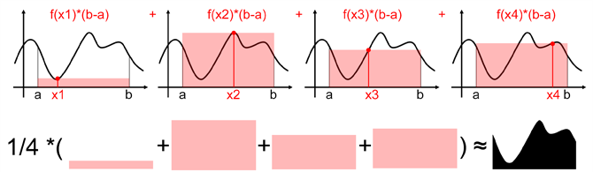
Monte Carlo Intergration

• It is too difficult to solve an integral analytically.
  • Thus estimate the integral of a function by averaging random samples of the function’s value.
• Different with Riemann integral which solve an integral analytically, Monte Carlo estimates the value of integration
• Define the Monte Carlo estimnator for the definite integral of given function $f(x)$
  • Definite integral
  \[\int_{a}^{b} f(x) d x\]
  • Random variable, where $p(x)$ is probability density function (pdf)
  \[X_{i} \sim p(x)\]
  • MonteCarlo estimator
  \[F_{N}=\frac{1}{N} \sum_{i=1}^{N} \frac{f\left(X_{i}\right)}{p\left(X_{i}\right)}\]

• Monte Carlo Integration

  \[\int f(x) dx = \frac{1}{N} \sum_{i=1}^{N} \frac{f\left(X_{i}\right)}{p\left(X_{i}\right)}\]
  • The more samples, the less variance
  • Sample on x, integrate on x
  • Don’t care about the domain of integration, but use numerical method sampling to estimate the value of integration
• When the random variable distributes between $a$ and $b$ uniformly

• Then the Basic Monte Carlo estimator will be

• If we want to keep the sampling number but increase the estimation accurarcy, we should sample from a distribution of interest than the uniform distribution, that is Importance Sampling

Path Tracing

Whitted-style problem

• Whitted-style ray tracing
  • Always perform specular reflections or refractions
  • Stop bouncing at diffuse surfaces

• But these simplifications are not reasonable

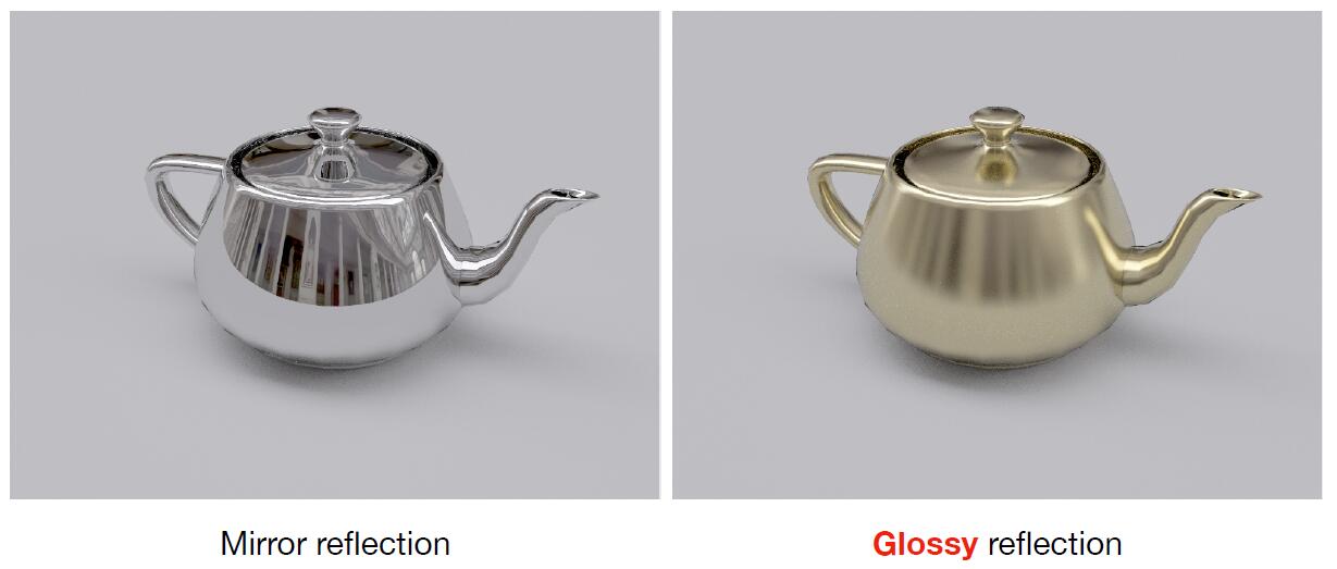
  • Whitted-style ray tracing can not deal with the glossy materials where the ray reflects not the same as the way on mirror material

  

  • Whitted-style ray tracing has no reflection between diffuse material

  

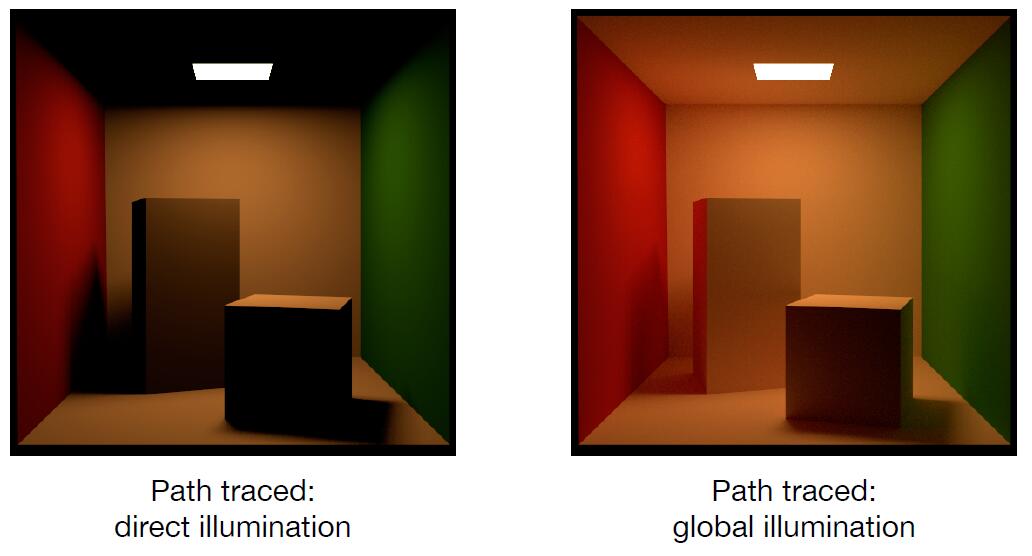
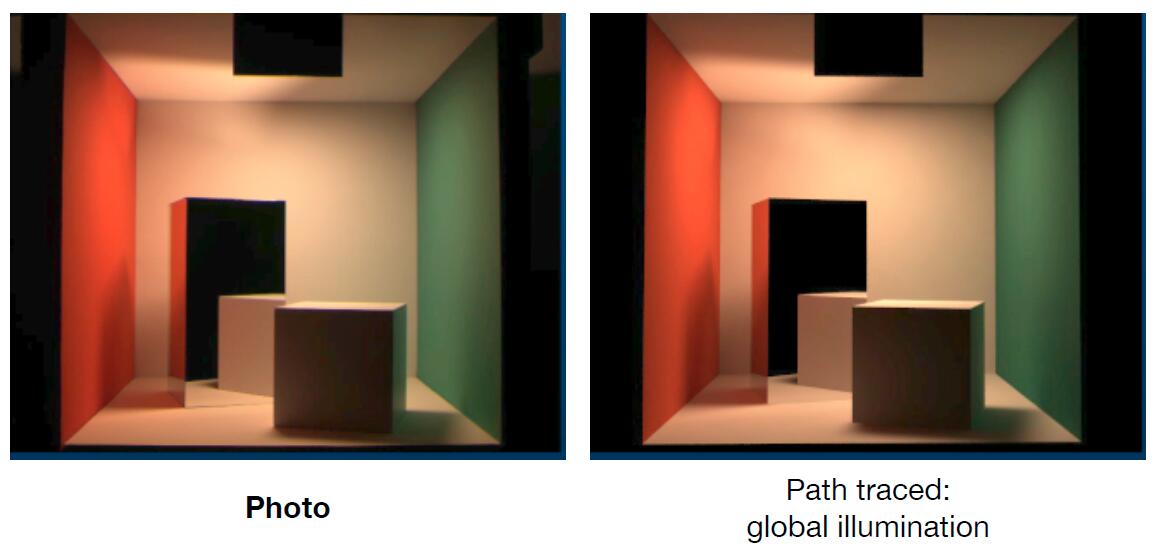
Tip: In the left image of the above figure, the region that are not reached by direct illumination are shadowed in black, whereas the diffuse ambient actually illuminates the region. In the right image, the left side of rectangular is shaded in red, and right side of cubic is shaded in green, This phenomenon in which objects or surfaces are colored by reflection of colored light from nearby surfaces is called color bleeding.

Solution of rendering equation

• The rendering equation to be solved

• It involves two problems
  • Solve an integral over the hemisphere
  • Deal with recursion of $L_{i}\left(p, \omega_{i}\right)$

A Sample Monte Carlo Solution

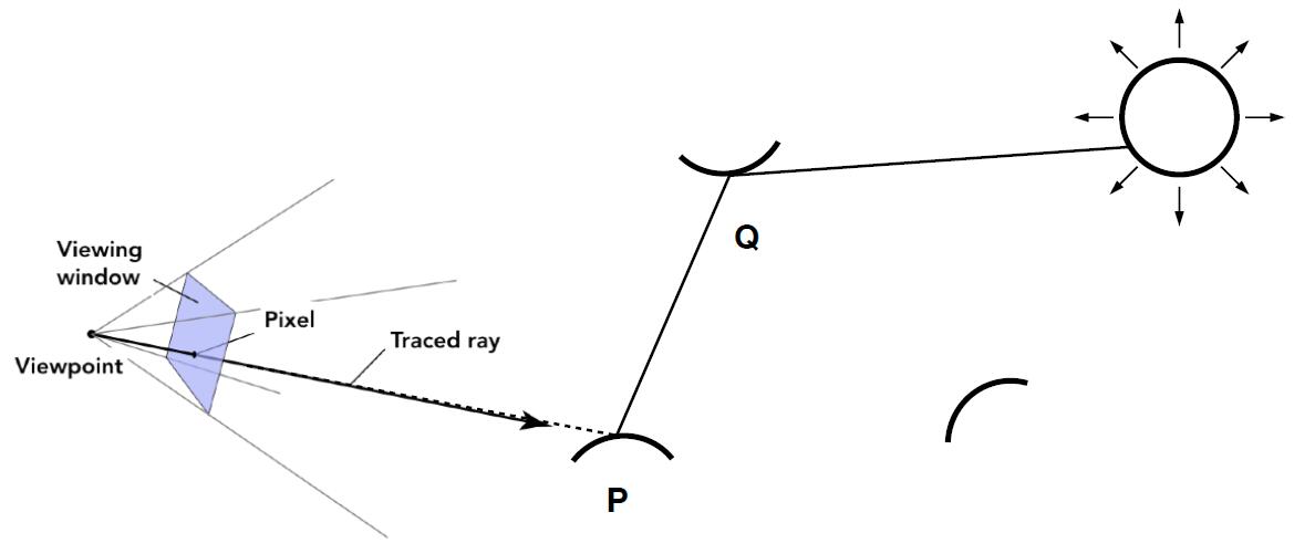
• Suppose we want to render one pixel (point) in the following scene for direct illumination only
  • No indirect reflection light is considered at this time

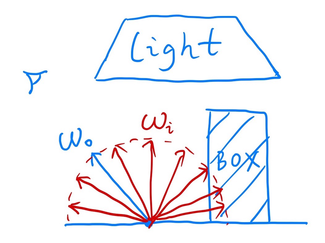
• Use Monte Carlo method to solve this integration numerically

  \[\int_{a}^{b} f(x) \mathrm{d} x \approx \frac{1}{N} \sum_{k=1}^{N} \frac{f\left(X_{k}\right)}{p\left(X_{k}\right)} \quad X_{k} \sim p(x)\]
  • $f(x)$: $L_{i}\left(p, \omega_{i}\right) f_{r}\left(p, \omega_{i}, \omega_{o}\right)\left(n \cdot \omega_{i}\right)$
  • $pdf$ (assume uniformly sampling the hemisphere): $pdf\left(\omega_{i}\right)=1 / 2 \pi$

• Shading algorithm for direct illumination

def shade(p, wo)
    Randomly choose **N** directions wi~pdf
    Lo = 0.0
    for each wi:
        Trace a ray r(p, wi)
        if ray r hit the light:
            Lo += (1 / N) * L_i * f_r * cosine / pdf(wi)
    return Lo

Introducing Global Illumination

• One more step forward: what if a ray hits an object
  • Point $Q$ also reflects light to $P$, and the amount of radiance is the amount of radiance of direct illumination at point $Q$

def shade(p, wo)
    Randomly choose **N** directions wi~pdf
    Lo = 0.0
    for each wi:
        Trace a ray r(p, wi)
        if ray r hit the light:
            Lo += (1 / N) * L_i * f_r * cosine / pdf(wi)
        # Add the following branch
        elif ray r hit an object at q:
            Lo += (1 / N) * shade(q, -wi) * f_r * cosine / pdf(wi)
            # minus wi is due to the reversed direction of the light towards object p
    return Lo

Problem 1: Number Explosion

• Explosion of num_rays as num_bounce goes up

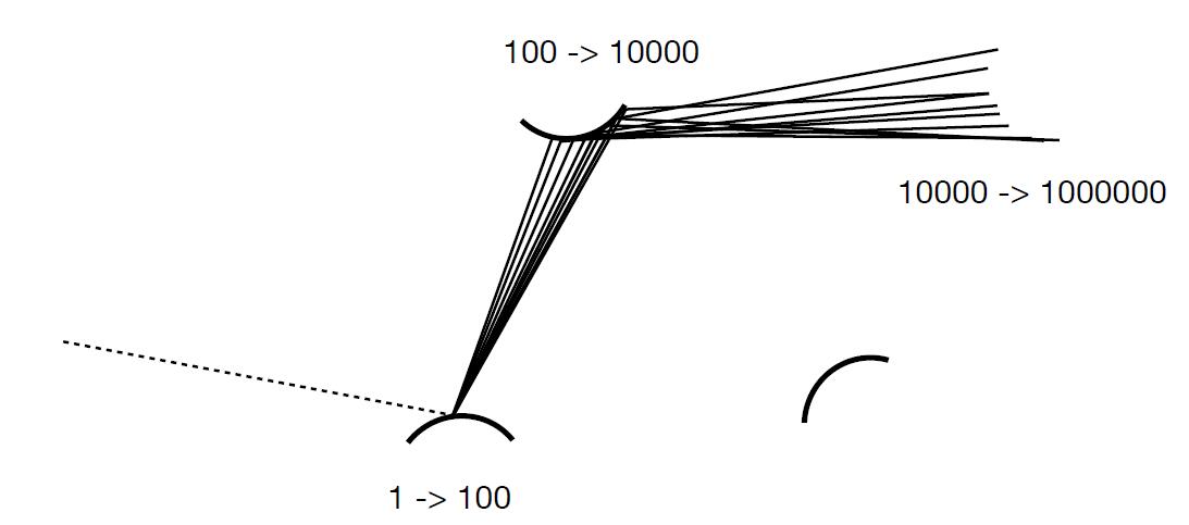
• num_ray will not explode if an only if $\color{red}{N = 1}$

• Path Tracing: only 1 ray is traced at each shading point

def shade(p, wo)
    #  modify N to One
    Randomly choose **One** directions wi~pdf
    Trace a ray r(p, wi)
    if ray r hit the light:
        return (1 / N) * L_i * f_r * cosine / pdf(wi)
    elif ray r hit an object at q:
        return (1 / N) * shade(q, -wi) * f_r * cosine / pdf(wi)

info: Distributed Ray Tracing: $ N != 1$

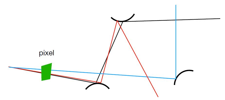
Ray Generation

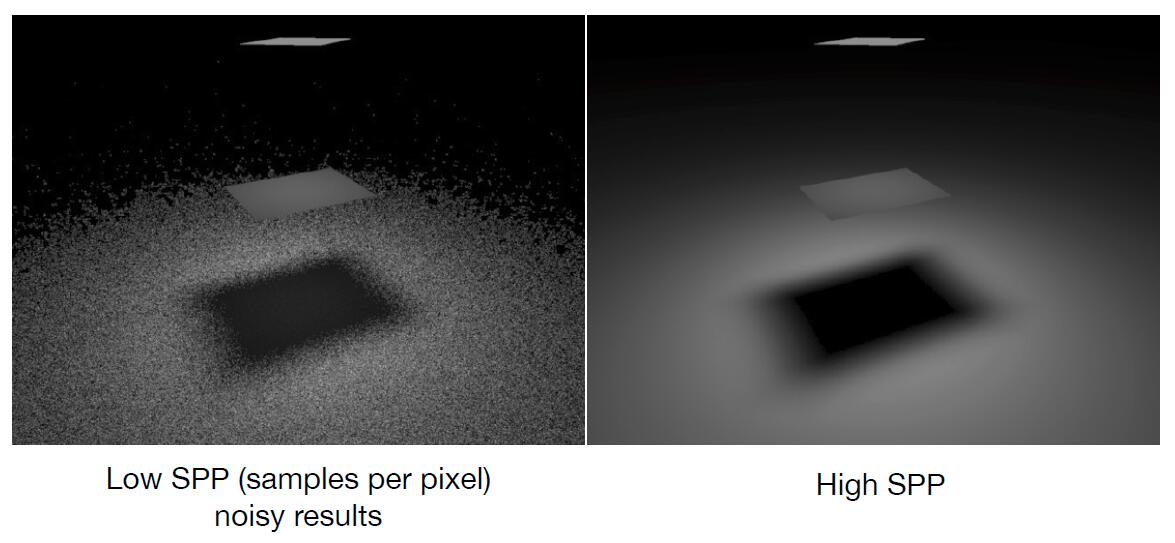
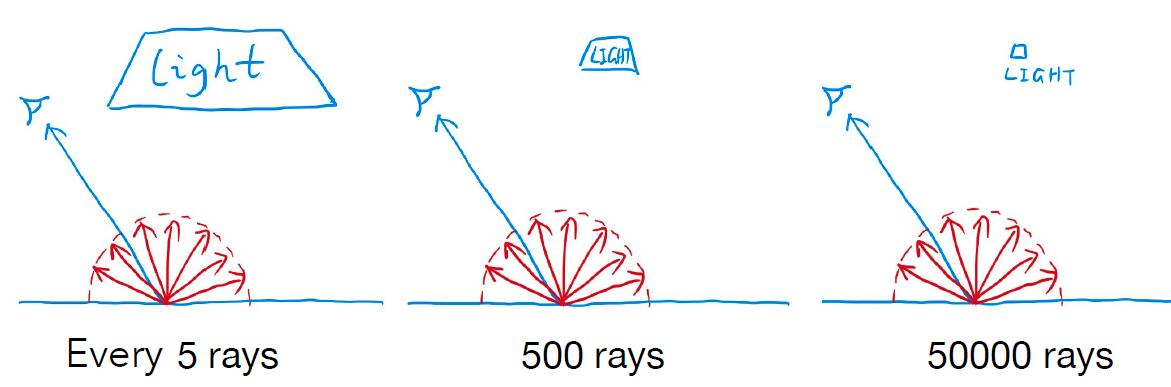
• If the ray is only sampled once, the shaded point will be noisy!
• BUT it doesn’t matter, because just trace more paths thorugh each pixel and average their radiance.
  • The goal is to render pixels of the image, instead of each points of objects in the scene.

def ray_generation(p, wo)
    Uniformly choose **N** sample positions within the pixel
    pixel_radiance = 0.0
    for each sample in the pixel:
        shoot a ray r(cam_pos, camera_to_sample)
        if ray r hit the scene at p:
            pixel_radiance += 1 / N * shade(p, - camera_to_sample)
    return pixel_radiance

Problem 2: Infinite Recursion

• Dilemma: the light does not stop bouncing indeed in the real world
• Further, cut num_bounce is to cut energy and reduce authenticity
• Solution: Russian Roulette (RR)
  • With probability $ 0 \lt P \lt 1$, condition 1
  • With probablity $1 - P$, otherwise
• Previously, we always shoot a ray at a shading point and get the shading result $L_o$
• Suppose we manually set a probability $P$
  • With probability $P$, shoot a ray and return the shading result divided by $P$: $L_o / P$
  • With probablity $1-P$, don’t shoot a ray and you’ll get $0$
• In this way, you can still expect to get $L_o$

def shade(p, wo)
    # Add the following branch
    Manually specify a probability p_RR
    Randomly select ksi in a uniform distribution in [0, 1]
    if ksi > p_RR:
        return 0.0
    Randomly choose **One** directions wi~pdf
    Trace a ray r(p, wi)
    if ray r hit the light:
        return (1 / N) * L_i * f_r * cosine / pdf(wi) / p_RR
    elif ray r hit an object at q:
        return (1 / N) * shade(q, -wi) * f_r * cosine / pdf(wi) / p_RR

• Expected value of bounce number, given probability $p$

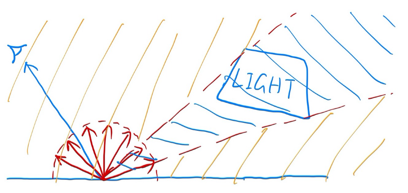
Sampling the Light

• Path tracing is correct but not efficient actually

• The reason of being inefficient is the sampled 1 ray may not hit the light, so that a lot of rays are wasted if we uniformly sample the hemisphere at the shading point

• Sampling on the shading point will lead to waste of rays which fail to hit the light source
  • Monte Carlo methods allows any sampling methods
  • Hence, change the sampling point to the light
• Assume uniformly sampling on the light

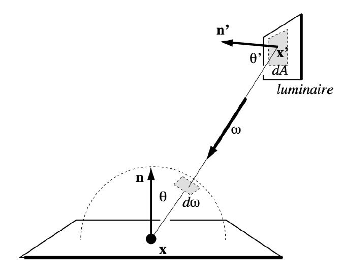
• The rendering equation integrates on the solid angle
  • Recall Monte Carlo Integration: Sample on $x$, and integrate on $x$
  • Integral variable substitution

• Make the rendering equation converting converting from an integral of $d\omega$ to $dA$.
• The relationship between $d\omega$ and $dA$
  • The projected area towards $x^\primex$ at point $x^\prime$ is $d A \cos \theta^{\prime}$
  • Recall that $dS = R^2d\theta$

Final Form of Path Tracing

• Rewrite the rendering equation as final form with an integral on $dA$

• Now integration is on the light, so for Monte Carlo integration:
  • $f(x)$ : $L_{i}\left(p, \omega_{i}\right) f_{r}\left(p, \omega_{i}, \omega_{o}\right) \frac{\cos \theta \cos \theta^{\prime}}{\left|x^{\prime}-x\right|^{2}}$
  • $pdf$ : $1 / A$
• Previously, we assume the light is accidentally shot by uniform hemisphere sampling
• Now we consider the radiance coming from two parts:
  • Light source (direct, no need to have RR), if the ray is not blocked in the middle
  • Other reflectors (indirect, need to have RR)

def shade(p, wo)
    # Contribution from the light source
    Uniformly sample the light at x' (pdf_light = 1 / A)
    L_dir = 0.0
    Shoot a ray from p to x'
    if the ray is not blocked in the middle:
        L_dir = Li * f_r * cosθ * cosθ' / |x' - p|^2 / pdf_light

    # Contribution from other reflections
    ## Test RR
    Manually specify a probability p_RR
    Randomly select ksi in a uniform distribution in [0, 1]
    if ksi > p_RR:
        return L_dir
    ## Ray Travce
    L_indir = 0.0
    Uniformly sample the hemisphere toward wi (pdf_hemi = 1 / 2pi)
    Trace a ray r(p, wi)
    if ray r hit a non-emitting object at q:
        L_indir = shade(q, -wi) * f_r * cosθ / pdf_hemi / p_RR
    return L_dir + L_indir

• Path tracing is almost 100% correct, a.k.a Photo-realistic

Summary & Future work

Summary

• Ray tracing: Previous vs. Modern Concepts
  • Previous: Ray tracing == Whitted-style ray tracing
  • Modern
    • The general solution of light transport, including:
    • (Unidirectional or Bidirectional) Path tracing
    • Photon mapping
    • Metropolis light transport
    • VCM / UPBP …

Future work

• Uniformly sampling the hemisphere
  • How? and in general, how to sample any function? (sampling theory)
• Monte Carlo integration allows arbitrary $pdf$
  • Instead of uniform sampling, what’s the best choice of sampling with regards to different shapes of function? (importance sampling)
• Do random numbers matter?
  • Yes! (low discrepancy sequences)
• I can sample the hemisphere and the light
  • Can I combine them? Yes! (multiple importance sampling)
• The radiance of a pixel is the averange of radiance on all paths passing through it
  • Why? If different weighted sampling at the center of pixel or the edge is needed? (pixel reconstruction filter)
• Is the radiance of a pixel the color of a pixel?
  • No. (gamma correction, curves concerning high dynamic range (HDR) image , color space, photography)

Reference

• GAMES101, Lingqi Yan
• 基于物理着色：BRDF
• 物理渲染(PBR)-基于物理的光照模型
• BRDF单位为sr^-1的原因
• Bi-Directional Reflectance Distribution Functions
• 蒙特·卡罗积分
• 蒙特卡洛积分概述
• 蒙特卡洛（Monte Carlo）法求定积分
• Rendering Equation求解